
Simpact Cyan - 0.19.3
This document is the reference documentation for the Simpact Cyan program, the C++ version of the Simpact family of programs. The program is most easily controlled through either the Python or R bindings, using the pysimpactcyan module and RSimpactCyan package respectively; the way to use them is described below. The Python bindings are included in the Simpact Cyan package, the R bindings need to be installed separately from within R.
Apart from this document, there exists some additional documentation as well:
- Documentation of the program code itself can be found here: code documentation.
- A tutorial for using the R bindings: Age-mixing tutorial Bruges 2015
The Simpact Cyan installers, as well as the source code for the program, can be found in the 'programs'. directory. If you're using MS-Windows, you'll need to install the Visual Studio 2013 redistributable package as well (use the x86 version) to be able to use the installed version.
In case you're interested in running simulations from R, you'll need to have a working Python version installed as well. For MS-Windows this is typically not installed by default; when installing this it's best to use the default directory (e.g. C:\Python27 or C:\Python34).
Introduction
Like other members of the Simpact family, Simpact Cyan is an agent based model (ABM) to study the way an infection spreads and can be influenced, and is currently focused on HIV. The program models each individual in a population of a specified initial size. Things that can happen are represented by events, which can have a certain risk of being executed at a certain moment. Time advances by iteratively finding the next event that will take place, updating the time to the corresponding value and executing event-specific code. The way this is implemented, is using the Modified Next Reaction Method [Anderson].
Note that event times and time-related properties that can be configured are expressed in units of years, unless stated otherwise.
Modified Next Reaction Method (mNRM) & hazards
In the mNRM algorithm, there is a core distinction between internal event times and real-world event times. The internal event times determine when an event will go off according to some notion of an internal clock. Let's call the internal time interval until a specific event fires \(\Delta T\). Such internal time intervals are chosen using a simple method, typically as random numbers picked from an exponential distribution:
\[ {\rm prob}(x)dx = \exp(-x)dx \]
Events in the simulation will not just use such internal times, they need to be executed at a certain real-world time. Calling \(\Delta t\) the real-world time interval that corresponds to the internal time interval \(\Delta T\), this mapping is done using the notion of a hazard (called propensity function in the mNRM article) \(h\):
\[ \Delta T = \int_{t_{\rm prev}}^{t_{\rm prev}+\Delta t} h(X(t'), t') dt' \]
It is this hazard that can depend on the state \(X\) of the simulation, and perhaps also explicitly on time. The state of the simulation in our case, can be thought of as the population: who has relationships with whom, who is infected, how many people are there etc. This state \(X(t)\) does not continuously depend on time: the state only changes when events get fired, which is when their internal time interval passes. Note that the formula above is for a single event, and while \(\Delta T\) itself is not affected by other events, the mapping into \(\Delta t\) certainly can be: other events can change the state, and the hazard depends on this state.
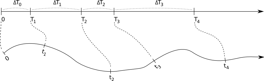
The figure below illustrates the main idea: internal time intervals are chosen from a certain distribution, and they get mapped onto real-world time intervals through hazards. Because hazards can depend both on the state (so the time until an event fires can be influenced by other events that manipulate this state), and can have an explicit time dependency, this mapping can be quite complex:
The hazard can cause complex behaviour, but of course this is not necessarily the case. If one uses a constant hazard, this simply causes a scaling between internal time \(\Delta T\) and real-world time \(\Delta t\): \[ \Delta T = h \Delta t \quad \text{(for a constant hazard)} \] This also illustrates that the higher the hazard, the earlier the event will fire, i.e. the real-world time interval will be smaller.
As an example, let's consider formation events. At a certain time in the simulation, many formation events will be scheduled, one event for each man/woman pair that can possibly form a relationship. The internal time interval for each of these events will simply be picked from the simple exponential distribution that was mentioned above. The mapping to a real-world time at which the event will fire, is calculated using the hazard-based method, and this hazard depends on many things (the state): how many relationships does the man have at a certain time, how many relationships does the woman have, what is the preferred age difference etc. One can also imagine that there can be an explicit time dependency in the hazard: perhaps the hazard of forming a relationship increases if the time since the relationship became possible goes up.
Using an exponential distribution to generate an internal time interval is how the method is described in the [Anderson] article. It is of course not absolutely necessary to do this, and other ways to generate an internal time are used as well. The simplest example, is if one wants to have an event that fires at a specific time. In that case, \(\Delta T\) can simply be set to the actual real-world time until the event needs to fire, and the hazard can be set to \(h=1\), so that internal and real-world time intervals match. Among others, this is done in the HIV seeding event which, when triggered, starts the epidemic by marking a certain amount of people as infected.
Population based simulation
Each time an event is triggered, the state of the simulation is allowed to change. Because the hazard of any event can depend on this state, in the most general version of the mNRM algorithm, one would recalculate the real-world event fire times of all remaining events each time a particular event gets triggered. This ensures that the possibly changed state is taken into account. Recalculating all event fire times all the time, is of course very inefficient: although the state may have been changed somewhat, this change may not be relevant for many of the event hazards in use. As a result, the calculated real-world fire times would be mostly the same as before.
In the Simpact model, the state can be thought of as the population that is being simulated, where the population consists of persons. Each person is linked to a list of events that involve him or her, and if an event is relevant to more than one person it will be present in the lists of more than one person. For example, a mortality event would be present in the list of only one person, while a relationship formation event is about two distinct people and would therefore be present in two such lists. The figure below illustrates this idea:
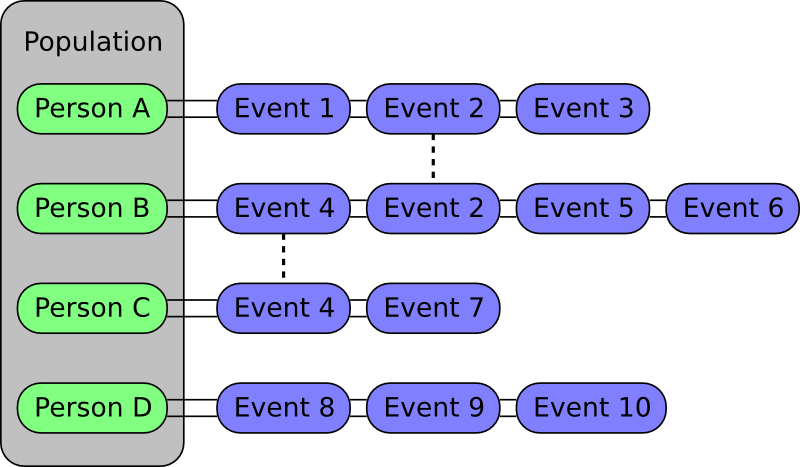
When an event fires, it is assumed that only the properties of a very limited set of people have changed, and that one only needs to recalculate the fire times of the events in those people's lists. For example, if Event 2 from the figure above fires, then the real-world fire times for the events in the lists of Person A and Person B will be automatically recalculated. Apart from affecting the people in whose lists an event appears, an event can also indicate that other people are affected. As an example, a birth event will only appear in the list of the woman who's pregnant. However, when triggered this event indicates that the father is also an affected person (in case the amount of children someone has is used in a hazard). In general, this number of other affected people will be very small compared to the size of the population, causing only a fraction of the event fire times to be recalculated. This allows this population-based algorithm to run much faster than the very basic algorithm that always recalculates all event times.
Besides these types of events, there are also 'global' events. These events do not refer to a particular person and will modify the state in a very general way. In general, when such a global event is triggered, this causes all other event fire times to be recalculated.
'Time limited' hazards
In the mNRM algorithm, time advances in steps, from one event fire time to the next. In general, these event fire times are calculated by mapping a generated internal time interval \(\Delta T\) onto a real-world time interval \(\Delta t\) using the formula
\[ \Delta T = \int_{t_{\rm prev}}^{t_{\rm prev}+\Delta t} h(X(t'), t') dt' \]
where \(h\) is the hazard that can have an explicit time dependency and a dependency on the simulation state. While the simulation state can change over time, it can only change at discrete points, when other events change the state.
The form of the hazard determines how fast this mapping between internal times and real-world times can be calculated. To keep the simulation as fast as possible, hazards for which the integral has an analytic solution are certainly most interesting. Furthermore, because the mapping between internal and real-world times needs to be done in each direction, the resulting equation for \(\Delta T\) needs to be invertible as well.
The hazards that we use in the Simpact events are often of the form
\[ {\rm hazard} = \exp(A+Bt) \]
This is a time dependent hazard where \(A\) and \(B\) are determined by other values in the simulation state. The nice feature of such a hazard is that it is always positive, as a hazard should be (otherwise the mapping could result in simulation time going backwards). Unfortunately, this form also has a flaw: consider the example where \(A = 0\), \(B = -1\) and \(t_{\rm prev} = 0\) for conciseness. The mapping between times then becomes
\[\Delta T = \int_0^{\Delta t} \exp(-t') dt' = 1 - \exp(-\Delta t) \]
When we need to map a specific \(\Delta t\) onto an internal \(\Delta T\), this expression can be used to do this very efficiently. When we need the reverse, rewriting this equation gives:
\[\Delta t = -\log(1-\Delta T) \]
From this it is clear that it is only possible if \(\Delta T\) is smaller than one, which may not be the case since \(\Delta T\) is picked from an exponential probability distribution in general. The core problem is that the integral in our expression is bounded, suggesting an upper limit on \(\Delta T\), but on the other hand that \(\Delta T\) needs to be able to have any positive value since it is picked from an exponential distribution which does not have an upper limit.
To work around this, we use a slightly different hazard, one that becomes constant after a certain time \(t_{\rm max}\), as is illustrated in the figure below. This has the effect that the integral will no longer have an upper bound, and the mapping from \(\Delta T\) to \(\Delta t\) will always be possible.
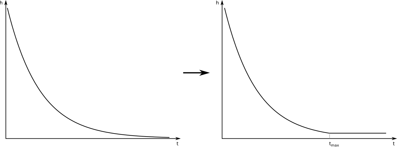
We are calculating a different hazard than before of course, so you may wonder whether this is really a good idea. In this respect, it is important to note that we're simulating individuals that will not live forever, but have a limited lifespan. So if we set \(t_{\rm max}\) to the time at which the relevant person would be 200 years old (for example), we can be very sure that our choice for \(t_{\rm max}\) will not affect the simulation. It only helps to keep the calculations feasible.
Above, the basic problem and solution are illustrated using a simple time dependent exponential hazard, but it should be clear that the problem occurs for other hazards as well: one only needs a hazard for which the integral above is bounded, and since choosing \(\Delta T\) from an exponential probability distribution can yield any value, problems will occur. The solution in the general case is the same: set the hazard to a constant value after a \(t_{\rm max}\) value which exceeds the lifetime of a person. The detailed calculations for this procedure can be found in this document: hazard_tmax.pdf
Configuration and running of a simulation
The basic Simpact Cyan program is a standalone command-line program. To be able to set up a simulation, you'd need to prepare a configuration file and specify this file as a command-line argument. Preparing the configuration file manually is time-consuming work, as all event properties necessary in a simulation need to be set. To make it easier to prepare and run simulations, there's a pysimpactcyan module that you can use to control Simpact Cyan from Python, or alternatively there's a RSimpactCyan library that you can install in R that provides a similar interface. The Python module is included when you install the Simpact Cyan binaries, the R library must be installed separately from an R session.
You can also use a combined approach: first run a simulation or simply prepare a configuration file from R or Python, and subsequently use this configuration to start one or more simulations. This can be very helpful to first prepare a base configuration file in an easy way, and then to launch one or more simulations on a computer cluster for example. For this particular case, it can be very helpful to override e.g. a prefix on the output files as explained below.
In this section, we briefly look into starting the simpact cyan program on the command line, followed by explanations of how the Python interface or R interface works. Some insights into the configuration file are given next, since that is the actual input to the simulation. Typically, if you can specify a particular probability distribution in the configuration file, you can also specify others. At the end of this section we describe which distributions are supported and what their parameters are.
Running from command line
The Simpact Cyan executable that you're likely to need is called simpact-cyan-release. There is a version with debugging information as well: this performs exactly the same calculations, but has more checks enabled. As a command line argument you can specify if the very basic mNRM (in which all event times are recalculated after triggering an event) is to be used, or the more advanced version (in which the program recalculates far less event fire times). While simpact-cyan-release with the advanced mNRM algorithm is the fastest, it may be a good idea to verify from time to time that the simple algorithm yields the same results (when using the same random number generator seed), as well as the debug versions.
The program needs three additional arguments, the first of which is the path to the configuration file that specifies what should be simulated. The configuration file is just a text file containing a list of key/value pairs, a part of which could look like this:
...
population.nummen    = 200
population.numwomen  = 200
population.simtime   = 40
...
You can also define variables and use environment variables of your system, later we'll look into this config file in more detail. All configuration options and their possible values are described in the section with the simulation details. For the configuration file itself, all options that are needed in the simulation must be set, no default values are assumed by the command line program. When using the R or Python interface however, this helper system does know about default values thereby severely limiting the number of options that must be specified. It will combine the options you specify with the defaults to produce a full configuration file that the command line program can use.
The second argument that the simpact-cyan-release program needs is either 0 or 1 and specifies whether the single core version should be used (corresponds to 0), or the version using multiple cores (corresponds to 1). For the parallel version, i.e. the version using multiple cores, OpenMP is used as the underlying technology. By default the program will try to use all processor cores your system has, but this can be adjusted by setting the OMP_NUM_THREADS environment variable. In general, it is a good idea to specify 0 for this option, selecting the single-core version. The parallel version currently only offers a modest speedup, and only for very large population sizes. Especially if you need to do several runs of a simulation, starting several single-core versions at once will use your computer's power more efficiently than starting several parallel versions in a sequential way.
With the third and final argument you can specify which mNRM algorithm to use: if you specify 'simple', the basic mNRM is used in which all event fire times will be recalculated after an event was triggered. Since this is a slow algorithm, you'll probably want to specify 'opt' here, to use the more advanced algorithm. In this case, the procedure explained above is used, where each user stores a list of relevant events.
So, assuming we've created a configuration file called myconfig.txt that resides in the current directory, we could run the corresponding simulation with the following command:
simpact-cyan-release myconfig.txt 0 optThis will produce some output on screen, such as which version of the program is being used and which random number generator seed was set. Since the random number generator seed is in there, it may be a good idea to save this to a file in case you'd like to reproduce the exact simulation later. To save it to a file called myoutput.txt, you can run
simpact-cyan-release myconfig.txt 0 opt 2>myoutput.txtNote that it is not a redirection of the output using simply >, but using 2>. This has to do with the fact that the information that you see on screen is actually sent to stderr instead of stdout.
When running the Simpact Cyan program, the default behaviour is to initialize the random number generator with a (more or less) random seed value. For reproducibility it may be necessary to enforce a specific seed. To do so, set the environment variable MNRM_DEBUG_SEED to the value you want to use, and verify in the output of the program that the specified seed is in fact the one being used:
for an MS-Windows system:
set MNRM_DEBUG_SEED=12345
simpact-cyan-release myconfig.txt 0 opt
Note that value of
MNRM_DEBUG_SEEDis still set, which is important when running additional simulations. To clear it, either exit the current command prompt, or executeset MNRM_DEBUG_SEED=(nothing may be specified after the
=sign, not even a space)for a Linux or OS X system:
export MNRM_DEBUG_SEED=12345
simpact-cyan-release myconfig.txt 0 opt
Note that value of
MNRM_DEBUG_SEEDis still set, which is important when running additional simulations. To clear it, either exit the current terminal window, or executeunset MNRM_DEBUG_SEEDOn one of these operating systems, it is also possible to specify everything in one line:
MNRM_DEBUG_SEED=12345 simpact-cyan-release myconfig.txt 0 optIn this case, the value of
MNRM_DEBUG_SEEDwill be visible to the program, but will no longer be set once the program finishes. It will therefore not affect other programs that are started.
Running from within R
Getting started
The R interface to Simpact Cyan will underneath still execute one of the Simpact Cyan programs, e.g. simpact-cyan-release, so the program relevant to your operating system must be installed first. Note that if you're using MS-Windows, you'll also need to install the Visual Studio 2013 redistributable package (use the x86 version).
The R module actually contains Python code so to be able to use this, you'll need to have a working Python installation. On Linux or OS X, this is usually already available, but if you're using MS-Windows you may need to install this separately. In this case, it is best to install it in the default directory, e.g. C:\Python27 or C:\Python34, so that the R package will be able to locate it easily.
Before being able to use the RSimpactCyan module, you need to make sure that other libraries are available:
install.packages("RJSONIO")
install.packages("findpython")
install.packages("rPithon", repos="http://research.edm.uhasselt.be/jori")
Once these are installed, you can install the RSimpactCyan library which contains the R interface to the Simpact Cyan program:
install.packages("RSimpactCyan", repos="http://research.edm.uhasselt.be/jori")Finally, you can load the library with the command:
library("RSimpactCyan")Running a simulation
To configure a simulation, you need to specify the options for which you want to use a value other than the default. This is done using a list, for example
cfg <- list()
cfg["population.nummen"] <- 200
cfg["population.numwomen"] <- 200
cfg["population.simtime"] <- 40
All values that are entered this way are converted to character strings when creating a configuration file for the simulation. This means that instead of a numeric value, you could also use a string that corresponds to the same number, for example
cfg["population.nummen"] <- "200"Together with the defaults for other options, these settings will be combined into a configuration file that the real Simpact Cyan program can understand. Taking a look at the full configuration file will show you what other values are in use; to see this configuration file, run
simpact.showconfig(cfg)Lines that start with a # sign are ignored when the configuration file is read. They may contain comments about certain options, or show which options are not in use currently. In case you'd want to use a simulation using all defaults, you can either use an empty list, or specify NULL.
If you've got the configuration you'd like to use, you can start the simulation from within R with the command simpact.run. Two parameters must be specified: the first is the settings to use (the cfg list in our example) and the second is a directory where generated files and results can be stored. The R module will attempt to create this directory if it does not exist yet. To use the directory /tmp/simpacttest, the command would become
res <- simpact.run(cfg, "/tmp/simpacttest")The other parameters are:
agedist: With this parameter, you can specify the age distribution that should be used when generating an initial population. The default is the age distribution of South Africa from 2003. In R, you can specify an alternative age distribution in two ways.The first way to do this, is to specify the age distribution as an R data frame or list, which contains columns named
Age,Percent.MaleandPercent.Female. TheAgecolumn should be increasing, and the other columns specify the probability of selecting each gender between the corresponding age and the next. Before the first specified age, this probability is zero, and the last mentioned age should have zeroes as the corresponding probabilities. The term probability here is not strictly correct: it can be any positive number since the resulting distribution will be normed. As an examplead <- list(Age=c(0,50,100), Percent.Male=c(1,2,0), Percent.Female=c(2,1,0))will correspond to an age distribution which limits the age to 100 for everyone. Furthermore, there will be twice as many men over 50 than under 50, while for the women it's the other way around.
The other way an age distribution can be specified, is as a CSV file with (at least) three columns. The header of this CSV file will not be taken into account, instead the first column is assumed to hold the
Agecolumn, the second is interpreted as thePercent.Malecolumn and the third asPercent.Female.intervention: With this simulation intervention setting it is possible to change configuration options that are being used at specific times during the simulation. More information about how this can be used can be found in the explanation of the simulation intervention event.release,slowalg,parallel: These flags specify which precise version of the simulation program will be used, and whether the single-core or multi-core version is used. Thereleaseparameter isTRUEby default, yielding the fastest version of the selected algorithm. If set toFALSE, many extra checks are performed, all of which should pass if the algorithm works as expected.By default,
slowalgisFALSEwhich selects the population-based procedure described above. In case this is set toTRUE, the very basic mNRM algorithm is used, where all event fire times are recalculated after each event is executed. If all works as expected, the two algorithms should produce the same results for the same seed (although very small differences are possible due to limited numeric precision). The basic algorithm is very slow, keep this in mind if you use it.The
parallelparameter isFALSEby default, selecting the version of the algorithm that only uses a single processor core. To use the parallel version, i.e. to use several processor cores at the same time, this can be set toTRUE. The parallel version currently only offers a modest speedup, and only for very large population sizes. Especially if you need to do several runs of a simulation, starting several single-core versions at once will use your computer's power more efficiently than starting several parallel versions in a sequential way.seed: By default, a more or less random seed value will be used to initialize the random number generator that's being using in the simulation. In case you'd like to use a specific value for the seed, for example to reproduce results found earlier, you can set it here.dryrun: If this is set toTRUE, the necessary configuration files will be generated, but the actual simulation is not performed. This can come in handy to prepare a simulation's settings on your local machine and run one or more actual simulations on another machine, e.g. on a computer cluster. In case you'd like to perform several runs with the same configuration file, overriding the output prefix can be very helpful, as is described in the section on the configuration file. If you'd like to perform a run that has been prepared this way from within R, you can use thesimpact.run.directfunction.identifierFormat: Files that are created by the simulation will all start with the same identifier. The identifierFormat parameter specifies what this identifier should be. Special properties start with a percent (%) sign, other things are just copied. An overview of these special properties:%T: will expand to the simulation type, e.g.simpact-cyan%y: the current year%m: the current month (number)%d: the current day of the month%H: the current hour%M: the current minute%S: the current second%p: the process ID of the process starting the simulation%r: a random character
The default identifier format
%T-%y-%m-%d-%H-%M-%S_%p_%r%r%r%r%r%r%r%r-would lead to an identifier likesimpact-cyan-2015-01-15-08-28-10_2425_q85z7m1G-.
The return value of the simpact.run function contains the paths to generated files and output files, or in case the dryrun option was used, of files that will be written to. The output files that are produced are described in the corresponding section.
Other functions
Apart from simpact.showconfig and simpact.run, some other functions exist in the RSimpactCyan library as well:
simpact.available
This function returns a boolean value, that indicates if theRSimpactCyanlibrary is able to find and use the Simpact Cyan simulation program.simpact.getconfig
This takes a list with config values as input, similar tosimpact.showconfig, merges it with default settings, and returns the extended configuration list. If the second parameter ('show') is set toTRUE, then the full configuration file will be shown on-screen as well.simpact.run.direct
This function allows you to start a simulation based on a previously created (e.g. using the 'dryrun' setting ofsimpact.run) configuration file. This config file must be set as the first argument, and is always required. Other arguments are optional:outputFile: If set toNULL, the output of the Simpact Cyan simulation (containing information about the version of the program and the random number generator seed) will just appear on screen. If a filename is specified here, the output will be written to that file as well.release,slowalg,parallel,seed: Same meaning as in thesimpact.runfunctiondestDir: By default, the simulation will be run in the directory that contains the config file. This is important if the config file itself specifies files without an absolute path name since the directory of the config file will then be used as a starting point. If you don't want this behaviour and need to select another directory, this parameter can be used to set it.
simpact.set.datadir
TheRSimpactCyanlibrary will try to figure out where the Simpact Cyan data files are located. If you want to specify another location, this function can be used to do so.simpact.set.simulation
The Simpact Cyan package is actually meant to support alternative simulations as well. To use such an alternative simulation, this function can be used. For example, ifmaxartis specified here, instead of running e.g.simpact-cyan-releaseas underlying program,maxart-releasewould be executed instead.
Running from within Python
Getting started
The pysimpactcyan module to control Simpact Cyan from within Python, is automatically available once you've installed the program. Note that if you're using MS-Windows, you'll also need to install the Visual Studio 2013 redistributable package (use the x86 version). To load the Simpact Cyan module in a Python script or interactive session, just execute
import pysimpactcyanThis allows you to create an instance of the PySimpactCyan class that's defined in this module, let's call it simpact:
simpact = pysimpactcyan.PySimpactCyan()Running a simulation
To configure a simulation, you need to specify the options for which you want to use a value other than the default. This is done using a dictionary, for example
cfg = { }
cfg["population.nummen"] = 200
cfg["population.numwomen"] = 200
cfg["population.simtime"] = 40
All values that are entered this way are converted to character strings when creating a configuration file for the simulation. This means that instead of a numeric value, you could also use a string that corresponds to the same number, for example
cfg["population.nummen"] = "200"Together with the defaults for other options, these settings will be combined into a configuration file that the real Simpact Cyan program can understand. Taking a look at the full configuration file will show you what other values are in use; to see this configuration file, run
simpact.showConfiguration(cfg)Lines that start with a # sign are ignored when the configuration file is read. They may contain comments about certain options, or show which options are not in use currently. In case you'd want to use a simulation using all defaults, you can either use an empty dictionary, or specify None.
If you've got the configuration you'd like to use, you can start the simulation from within Python using the run method of the Simpact Cyan object you're using. Two parameters must be specified: the first is the settings to use (the cfg dictionary in our example) and the second is a directory where generated files and results can be stored. The Python module will attempt to create this directory if it does not exist yet. To use the directory /tmp/simpacttest, the command would become
res = simpact.run(cfg, "/tmp/simpacttest")The other parameters are:
agedist: With this parameter, you can specify the age distribution that should be used when generating an initial population. The default is the age distribution of South Africa from 2003. In Python, you can specify an alternative age distribution in two ways.The first way to do this, is to specify the age distribution as a dictionary which contains lists of numbers named
Age,Percent.MaleandPercent.Female. TheAgelist should be increasing, and the other lists specify the probability of selecting each gender between the corresponding age and the next. Before the first specified age, this probability is zero, and the last mentioned age should have zeroes as the corresponding probabilities. The term probability here is not strictly correct: it can be any positive number since the resulting distribution will be normed. As an examplead = { "Age": [0, 50, 100], "Percent.Male": [1, 2, 0], "Percent.Female": [2, 1, 0] }will correspond to an age distribution which limits the age to 100 for everyone. Furthermore, there will be twice as many men over 50 than under 50, while for the women it's the other way around.
The other way an age distribution can be specified, is as a CSV file with (at least) three columns. The header of this CSV file will not be taken into account, instead the first column is assumed to hold the
Agecolumn, the second is interpreted as thePercent.Malecolumn and the third asPercent.Female.parallel,opt,release: These flags specify which precise version of the simulation program will be used, and whether the single-core or multi-core version is used. Thereleaseparameter isTrueby default, yielding the fastest version of the selected algorithm. If set toFalse, many extra checks are performed, all of which should pass if the algorithm works as expected.By default,
optisTruewhich selects the population-based procedure described above. In case this is set toFalse, the very basic mNRM algorithm is used, where all event fire times are recalculated after each event is executed. If all works as expected, the two algorithms should produce the same results for the same seed (although very small differences are possible due to limited numeric precision). The basic algorithm is very slow, keep this in mind if you use it.The
parallelparameter isFalseby default, selecting the version of the algorithm that only uses a single processor core. To use the parallel version, i.e. to use several processor cores at the same time, this can be set toTrue. The parallel version currently only offers a modest speedup, and only for very large population sizes. Especially if you need to do several runs of a simulation, starting several single-core versions at once will use your computer's power more efficiently than starting several parallel versions in a sequential way.seed: By default, a more or less random seed value will be used to initialize the random number generator that's being using in the simulation. In case you'd like to use a specific value for the seed, for example to reproduce results found earlier, you can set it here.interventionConfig: With this simulation intervention setting it is possible to change configuration options that are being used at specific times during the simulation. More information about how this can be used can be found in the explanation of the simulation intervention event.dryRun: If this is set toTrue, the necessary configuration files will be generated, but the actual simulation is not performed. This can come in handy to prepare a simulation's settings on your local machine and run one or more actual simulations on another machine, e.g. on a computer cluster. In case you'd like to perform several runs with the same configuration file, overriding the output prefix can be very helpful, as is described in the section on the configuration file. If you'd like to perform a run that has been prepared this way from within Python, you can use therunDirectmethod of thePySimpactCyanclass.identifierFormat: Files that are created by the simulation will all start with the same identifier. The identifierFormat parameter specifies what this identifier should be. Special properties start with a percent (%) sign, other things are just copied. An overview of these special properties:%T: will expand to the simulation type, e.g.simpact-cyan%y: the current year%m: the current month (number)%d: the current day of the month%H: the current hour%M: the current minute%S: the current second%p: the process ID of the process starting the simulation%r: a random character
The default identifier format
%T-%y-%m-%d-%H-%M-%S_%p_%r%r%r%r%r%r%r%r-would lead to an identifier likesimpact-cyan-2015-01-15-08-28-10_2425_q85z7m1G-.
The return value of the run method contains the paths to generated files and output files, or in case the dryRun option was used, of files that will be written to. The output files that are produced are described in the corresponding section.
Other functions
Apart from the PySimpactCyan methods showConfiguration and run, some other methods exist in this Python class as well:
getConfiguration
This takes a dictionary with config values as input, similar toshowConfiguration, merges it with default settings, and returns the extended configuration dictionary. If the second parameter ('show') is set toTrue, then the full configuration file will be shown on-screen as well.runDirect
This function allows you to start a simulation based on a previously created (e.g. using the 'dryRun' setting ofrun) configuration file. This config file must be set as the first argument, and is always required. Other arguments are optional:outputFile: If set toNone, the output of the Simpact Cyan simulation (containing information about the version of the program and the random number generator seed) will just appear on screen. If a filename is specified here, the output will be written to that file as well.release,opt,parallel,seed: Same meaning as in therunmethod.destDir: By default, the simulation will be run in the directory that contains the config file. This is important if the config file itself specifies files without an absolute path name since the directory of the config file will then be used as a starting point. If you don't want this behaviour and need to select another directory, this parameter can be used to set it.
setSimpactDataDirectory
Thepysimpactcyanmodule will try to figure out where the Simpact Cyan data files are located. If you want to specify another location, this function can be used to do so.setSimpactDirectory
In case you want to specify that the Simpact Cyan executables are located in a specific directory, you can use this function.setSimulationPrefixThe Simpact Cyan package is actually meant to support alternative simulations as well. To use such an alternative simulation, this function can be used. For example, ifmaxartis specified here, instead of running e.g.simpact-cyan-releaseas underlying program,maxart-releasewould be executed instead.
Configuration file and variables
The actual program that executes the simulation reads its settings from a certain configuration file. This is also the case when running from R or Python, where the R or Python interface prepares the configuration file and executes the simulation program. While this approach makes it much easier to configure and run simulations, some knowledge of the way the configuration file works can be helpful.
The basics
In essence, the configuration file is just a text file containing key/value pairs. For example, the line
population.simtime = 100assigns the value 100 to the simulation setting population.simtime, indicating that the simulation should run for 100 years. Lines that start with a hash sign (#) are not processed, they can be used for comments. In the config file itself, mathematical operations are not possible, but if you're using R or Python, you can perform the operation there, and only let the result appear in the config file. For example, if you'd do
library("RSimpactCyan")
cfg <- list()
cfg["population.simtime"] = 100/4
simpact.showconfig(cfg)
in an R session, you'd find
population.simtime = 25in the configuration file. We could force '100/4' to appear in the configuration file by changing the line to
cfg["population.simtime"] = "100/4"(so we added quotes), but when trying to run the simulation this would lead to the following error:
FATAL ERROR:
Can't interpret value for key 'population.simtime' as a floating point number
Config file variables and environment variables
Keys that start with a dollar sign ($) are treated in a special way: they define a variable that can be used further on in the configuration file. To use a variable's contents in the value part of a config line, the variable's name should be placed between ${ and }. For example, we could first have set
$SIMTIME = 100thereby assigning 100 to the variable with name SIMTIME. This could then later be used as follows:
population.simtime = ${SIMTIME}You don't even need to define the variable inside the configuration file: if you define an environment variable, you can use its contents in the same way as before. For example, if the HOME environment variable has been set to /Users/JohnDoe/, then the lines
periodiclogging.interval            = 2
periodiclogging.outfile.logperiodic = ${HOME}periodiclog.csv
would enable the periodic logging event and write its output every other year to /Users/JohnDoe/periodiclog.csv.
One very important thing to remember is that if an environment variable with the same name as a config file variable exists, the environment variable will always take precedence over config file variables. While this might seem a bit odd, it actually allows you to more easily use config files prepared on one system, on another system. Furthermore, it allows you to use a single config file multiple times, which can be very handy if you need to perform many runs using the same settings (but different output files).
Using environment variables
When you let the R or Python interface prepare a configuration file, this file will start by defining two config file variables, for example:
$SIMPACT_OUTPUT_PREFIX = simpact-cyan-2015-05-27-08-28-13_27090_8Al7O6mD-
$SIMPACT_DATA_DIR = /usr/local/share/simpact-cyan/
The first variable is used in the config file when specifying which files to write output to. As an example, you'd also find the line
logsystem.outfile.logevents = ${SIMPACT_OUTPUT_PREFIX}eventlog.csvin that file, so the full output file name would be
simpact-cyan-2015-05-27-08-28-13_27090_8Al7O6mD-eventlog.csvThe second variable specifies the location that R or Python thinks the Simpact Cyan data files are stored in, and is used in the line that specifies which age distribution to use when initializing the population:
population.agedistfile = ${SIMPACT_DATA_DIR}sa_2003.csvIn this case, the file /usr/local/share/simpact-cyan/sa_2003.csv would be used to read the initial age distribution from.
Because those config variables are defined inside the configuration file, such a file can be used on its own. If you'd first prepared the config file using the 'dryrun' setting, you could still use the created config file to start the simulation, either directly on the command line, using simpact.run.direct from R, or using the PySimpactCyan method runDirect in Python.
If you're running from the command line, it's very easy to reuse the same configuration file for multiple runs. Normally if you'd try this, you'd see an error message like
FATAL ERROR:
Unable to open event log file:
Specified log file simpact-cyan-2015-05-27-08-28-13_27090_8Al7O6mD-eventlog.csv already exists
To make sure that you don't lose data from simulations you've already performed, the simulation will not start if it needs to overwrite an output file, which is what causes this message.
However, because we can easily override the value of SIMPACT_OUTPUT_PREFIX from the command line by using an environment variable with the same name, it becomes possible to reuse the configuration file multiple times. For example, assuming that our config file is called myconfig.txt, the simple bash script
for i in 1 2 3 4 5 ; do
    SIMPACT_OUTPUT_PREFIX=newprefix_${i}- simpact-cyan-release myconfig.txt 0 opt
done
would produce output files like newprefix_1-eventlog.csv and newprefix_5-eventlog.csv.
In a similar way, setting an environment variable called SIMPACT_DATA_DIR can be helpful when preparing simulations on one system and running them on another. For example, you could prepare the simulations on your laptop, using the 'dryrun' option to prevent the simulation from actually running, and execute them on e.g. a computer cluster where you set the SIMPACT_DATA_DIR environment variable to make sure that the necessary data files can still be found.
Supported probability distributions and their parameters
If a configuration option ends with .dist.type or .dist2d.type, for example option birth.pregnancyduration.dist.type of the birth event, you can specify a number of probability distributions there. By choosing a specific type of probability distribution, you also activate a number of other options to configure the parameters of this probability distribution.
For example, if birth.pregnancyduration.dist.type is set to normal, then parameters of the one dimensional normal distribution need to be configured. For example, we could set birth.pregnancyduration.dist.normal.mu to 0.7342 and birth.pregnancyduration.normal.sigma to 0.0191, and we'd get a birth event that on average takes place after 0.7342 years (is 268 days), with a standard deviation of roughly one week (0.0191 years).
Below you can find an overview of the currently supported one and two dimensional distributions and their parameters.
One dimensional distributions
Here is an overview of the relevant configuration options, their defaults (between parentheses), and their meaning:
some.option.dist.type: ('fixed'):
With such an option, you specify which specific distribution to choose. Allowed values arebeta,exponential,fixed,gamma,lognormal,normal,uniform, and the corresponding parameters are given in the subsections below. Unless otherwise specified, the default here is afixeddistribution, which is not really a distribution but just causes a fixed value to be used.
beta
If this distribution is chosen, the (scaled) beta distribution with the following probability density is used:
\[ {\rm prob}(x) = \frac{\Gamma(a+b)}{\Gamma(a)\Gamma(b)} \left(\frac{x-x_{\rm min}}{x_{\rm max}-x_{\rm min}}\right)^{a-1} \left(1-\frac{x-x_{\rm min}}{x_{\rm max}-x_{\rm min}}\right)^{b-1} \frac{1}{x_{\rm max}-x_{\rm min}} \]
This corresponds to a beta distribution that, instead of being non-zero between 0 and 1, is now scaled and translated to be defined between \(x_{\rm min}\) and \(x_{\rm max}\).
Here is an overview of the relevant configuration options, their defaults (between parentheses), and their meaning:
some.option.dist.beta.a(no default):
Corresponds to the value of \(a\) in the formula for the probability density above.some.option.dist.beta.b(no default):
Corresponds to the value of \(b\) in the formula for the probability density above.some.option.dist.beta.max(no default):
Corresponds to the value of \(x_{\rm min}\) in the formula for the probability density above.some.option.dist.beta.min(no default):
Corresponds to the value of \(x_{\rm max}\) in the formula for the probability density above.
exponential
If the exponential distribution is selected, the probability density for a negative value is zero, while the probability density for positive values is given by:
\[ {\rm prob}(x) = \lambda \exp(-\lambda x) \]
Here is an overview of the relevant configuration options, their defaults (between parentheses), and their meaning:
some.option.dist.exponential.lambda(no default):
This specifies the value of \(\lambda\) in the expression of the probability density above.
fixed
This does not really correspond to a distribution, instead a predefined value is always used.
Here is an overview of the relevant configuration options, their defaults (between parentheses), and their meaning:
some.option.dist.fixed.value(0):
When a number is chosen from this 'distribution', this value is always returned.
gamma
In this case, the gamma distribution will be used to choose random numbers. The probability density is
\[ {\rm prob}(x) = \frac{x^{a-1} \exp\left(-\frac{x}{b}\right)}{b^a \Gamma(a)} \]
for positive numbers, and zero for negative ones.
Here is an overview of the relevant configuration options, their defaults (between parentheses), and their meaning:
some.option.dist.gamma.a(no default):
This corresponds to the value of \(a\) in the expression of the probability distribution.some.option.dist.gamma.b(no default):
This corresponds to the value of \(b\) in the expression of the probability distribution.
lognormal
If this log-normal distribution is chosen, the probability density for negative numbers is zero, while for positive numbers it is:
\[ {\rm prob}(x) = \frac{1}{x \sigma \sqrt{2\pi}} \exp\left(-\frac{(\log{x}-\zeta)^2}{2\sigma^2}\right) \]
Here is an overview of the relevant configuration options, their defaults (between parentheses), and their meaning:
some.option.dist.lognormal.sigma(no default):
This corresponds to the value of \(\sigma\) in the formula for the probability distribution.some.option.dist.lognormal.zeta(no default):
This corresponds to the value of \(\zeta\) in the formula for the probability distribution.
normal
The base probability distribution used when the normal distribution is selected is the following:
\[ {\rm prob}(x) = \frac{1}{\sigma\sqrt{2\pi}} \exp\left(- \frac{(x-\mu)^2}{2\sigma^2}\right) \]
It is possible to specify a minimum and maximum value as well, which causes the probability density to be zero outside of these bounds, and somewhat higher in between. A very straightforward rejection sampling method is used for this at the moment, so it is best not to use this to sample from a narrow interval (or in general an interval with a low probability) since this can require many iterations.
Here is an overview of the relevant configuration options, their defaults (between parentheses), and their meaning:
some.option.dist.normal.max(+infinity):
This can be used to specify the maximum value beyond which the probability density is zero. By default no truncation is used, and this maximum is set to positive infinity.some.option.dist.normal.min(-infinity):
This can be used to specify the minimum value below which the probability density is zero. By default no trunctation is used, and this minimum is set to negative infinity.some.option.dist.normal.mu(no default):
This corresponds to the value of \(\mu\) in the expression of the probability density above.some.option.dist.normal.sigma(no default):
This corresponds to the value of \(\sigma\) in the expression of the probability density above.
uniform
When this probability density is selected, each number has an equal probability density between a certain minimum and maximum value. Outside of these bounds, the probability density is zero.
Here is an overview of the relevant configuration options, their defaults (between parentheses), and their meaning:
some.option.dist.uniform.min(0):
This specifies the start of the interval with the same, constant probability density.some.option.dist.uniform.max(1):
This specifies the end of the interval with the same, constant probability density.
Two dimensional distributions
Here is an overview of the relevant configuration options, their defaults (between parentheses), and their meaning:
some.option.dist2d.type('fixed'):binormal,binormalsymm,discrete,fixed,uniform
binormal
This corresponds to the two dimensional multivariate normal distribution, which has the following probability density:
\[ {\rm prob}(x,y) = \frac{1}{2\pi\sigma_x\sigma_y\sqrt{1-\rho^2}} \exp\left[-\frac{ \frac{(x-\mu_x)^2}{\sigma_x^2} + \frac{(y-\mu_y)^2}{\sigma_y^2} - \frac{2\rho (x-\mu_x)(y-\mu_y)}{\sigma_x\sigma_y} }{2(1-\rho^2)} \right] \]
If desired, this probability density can be truncated to specific bounds, by setting the minx, maxx, miny and maxy parameters. These default to negative and positive infinity causing truncation to be disabled. To enforce these bounds a straightforward rejection sampling method is used, so to avoid a large number of iterations to find a valid random number, it is best not to restrict the acceptable region to one with a low probability.
Here is an overview of the relevant configuration options, their defaults (between parentheses), and their meaning:
some.option.dist2d.binormal.meanx(0):
Corresponds to \(\mu_x\) in the expression for the probability density above.some.option.dist2d.binormal.meany(0):
Corresponds to \(\mu_y\) in the expression for the probability density above.some.option.dist2d.binormal.rho(0):
Corresponds to \(\rho\) in the expression for the probability density above.some.option.dist2d.binormal.sigmax(1):
Corresponds to \(\sigma_x\) in the expression for the probability density above.some.option.dist2d.binormal.sigmay(1):
Corresponds to \(\sigma_y\) in the expression for the probability density above.some.option.dist2d.binormal.minx(-infinity):
This can be used to truncate the probability distribution in the x-direction.some.option.dist2d.binormal.maxx(+infinity):
This can be used to truncate the probability distribution in the x-direction.some.option.dist2d.binormal.miny(-infinity):
This can be used to truncate the probability distribution in the y-direction.some.option.dist2d.binormal.maxy(+infinity):
This can be used to truncate the probability distribution in the y-direction.
binormalsymm
This is similar to the binormal distribution above, but using the same parameters for the x-direction as for the y-direction. This means it is also a two dimensional multivariate normal distribution, but with a less general probability distribution:
\[ {\rm prob}(x,y) = \frac{1}{2\pi\sigma^2\sqrt{1-\rho^2}} \exp\left[-\frac{(x-\mu)^2 + (y-\mu)^2 - 2\rho (x-\mu)(y-\mu)}{2\sigma^2 (1-\rho^2)}\right] \]
If desired, this probability density can be truncated to specific bounds, by setting the min and max parameters. These default to negative and positive infinity causing truncation to be disabled. To enforce these bounds a straightforward rejection sampling method is used, so to avoid a large number of iterations to find a valid random number, it is best not to restrict the acceptable region to one with a low probability.
Here is an overview of the relevant configuration options, their defaults (between parentheses), and their meaning:
some.option.dist2d.binormalsymm.mean(0):
This corresponds to the value of \(\mu\) in the formula for the probability density.some.option.dist2d.binormalsymm.rho(0:
This corresponds to the value of \(\rho\) in the formula for the probability density.some.option.dist2d.binormalsymm.sigma(1):
This corresponds to the value of \(\sigma\) in the formula for the probability density.some.option.dist2d.binormalsymm.max(+infinity):
This can be used to truncate the probability density, to set a maximum in both the x- and y-directions.some.option.dist2d.binormalsymm.min(-infinity):
This can be used to truncate the probability density, to set a minimum in both the x- and y-directions.
discrete
With the discrete distribution, you can use a TIFF image file to specify a probability distribution. This can come in handy if you'd like to use population density data for example. The TIFF file format is very general, and can support several sample representations and color channels. Since the specified file will be used for a probability distribution, only one value per pixel is allowed (as opposed to separate values for red, green and blue for example), and a 32-bit or 64-bit floating point representation should be used. Negative values are set to zero, while positive values will be normalized and used for the probability distribution.
If desired, a 'mask file' can be specified as well (using maskfile). Such a file should also be a TIFF file, with the same number of pixels in each dimension. If the value of a certain pixel in the mask file is zero or negative, the value read from the real input file (densfile) will be set to zero, otherwise the value from the real input file is left unmodified. This can be used to easily restrict the original file to a certain region.
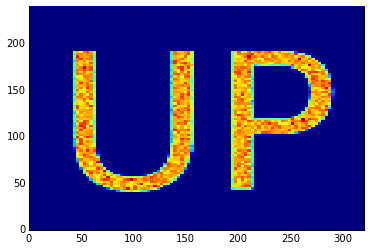
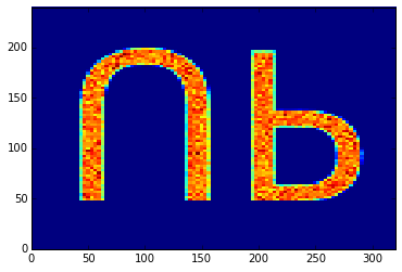
Suppose we have an 320x240 image that we'd like to use to base a probability density on. In the TIFF file format, as with many other image formats, the upper-left pixel is the (0, 0) pixel, while the bottom-right pixel will be (319, 239). Usually, we'd like the y-axis to point up however, which is why the default value of the flipy parameter is set to yes. To illustrate, suppose we use the up32.tiff file, which corresponds to the following image. If we use this as a discrete probability density, a histogram of the samples should show the text 'UP'.

In the discretedistribution.ipynb example, we abuse the setting of the population density to sample from this distribution: each person will have a location that is sampled from this discrete distribution. In case the flipy parameter is yes (the default), we obtain the following histogram, which is probably what we'd expect.
On the other hand, if we explicitly set the flipy parameter to no, the mismatch between the y-axes becomes apparent:
The image file itself just specifies the shape of the probability distribution. The actual size and position in the x-y plane can be set using the width, height xoffset and yoffset parameters.
Here is an overview of the relevant configuration options, their defaults (between parentheses), and their meaning:
some.option.dist2d.discrete.densfile(no default):
This should be used to specify the TIFF file that contains the discrete probability density to be used.some.option.dist2d.discrete.maskfile(no default):
As explained above, a TIFF mask file can be used to restrict the previous file to a certain region. Set to an empty string in case you don't need this.some.option.dist2d.discrete.flipy('yes'):
By default, the image will be flipped in the y-direction. This has to do with the y-axis in images being different from what we'd expect (see explanation above).some.option.dist2d.discrete.width(1):
The TIFF file itself just specifies the shape of the distribution. With this parameter you can set the actual width (scale in x-direction) in the x-y plane.some.option.dist2d.discrete.height(1):
The TIFF file itself just specifies the shape of the distribution. With this parameter you can set the actual height (scale in y-direction) in the x-y plane.some.option.dist2d.discrete.xoffset(0):
The TIFF file itself just specifies the shape of the distribution. With this parameter you can set the x-offset in the x-y plane.some.option.dist2d.discrete.yoffset(0):
The TIFF file itself just specifies the shape of the distribution. With this parameter you can set the y-offset in the x-y plane.
fixed
This does not really correspond to a distribution, instead a predefined (x, y) value is always used.
Here is an overview of the relevant configuration options, their defaults (between parentheses), and their meaning:
some.option.dist2d.fixed.xvalue(0):
The x-value of the (x, y) coordinate that is always returned.some.option.dist2d.fixed.yvalue(0):
The y-value of the (x, y) coordinate that is always returned.
uniform
By specifying this probability density, a point shall be chosen from a rectangular region in the x-y plane. All points within this region have an equal probability density, while points outside the region have a probably density of zero.
Here is an overview of the relevant configuration options, their defaults (between parentheses), and their meaning:
some.option.dist2d.uniform.xmin(0):
This specifies the start of the region along the x-axis.some.option.dist2d.uniform.xmax(1):
This specifies the end of the region along the x-axis.some.option.dist2d.uniform.ymin(0):
This specifies the start of the region along the y-axis.some.option.dist2d.uniform.ymax(1):
This specifies the end of the region along the y-axis.
Output
By default, four log files are used, but they can be disabled by assigning an empty string to the configuration property. If you're using the R or Python interface, the full paths of these log files will be stored in the object returned by simpact.run or the PySimpactCyan method run.
Here is an overview of the relevant configuration options, their defaults (between parentheses), and their meaning:
logsystem.outfile.logevents('${SIMPACT_OUTPUT_PREFIX}eventlog.csv'):
Here, all events that take place are logged. See the section about the configuration file for additional information regarding theSIMPACT_OUTPUT_PREFIXvariable.logsystem.outfile.logpersons('${SIMPACT_OUTPUT_PREFIX}personlog.csv'):
In this file, information about every person in the simulation is stored. See the section about the configuration file for additional information regarding theSIMPACT_OUTPUT_PREFIXvariable.logsystem.outfile.logrelations('${SIMPACT_OUTPUT_PREFIX}relationlog.csv'):
Here, all relationships are logged. See the section about the configuration file for additional information regarding theSIMPACT_OUTPUT_PREFIXvariable.logsystem.outfile.logtreatments('${SIMPACT_OUTPUT_PREFIX}treatmentlog.csv'):
This file records information regarding treatments. See the section about the configuration file for additional information regarding theSIMPACT_OUTPUT_PREFIXvariable.
Event log
The event log is a CSV-like file, in which each line contains at least ten entries:
- The simulation time at which the event took place
- A short description of the event
- The name of the first person involved in the event, or
(none) - The person ID of the first person involved, or -1
- The gender (0 for a man, 1 for a woman) of the first person involved in the event, or -1
- The age of the first person involved in the event, or -1
- The name of the second person involved in the event, or
(none) - The person ID of the second person involved, or -1
- The gender (0 for a man, 1 for a woman) of the second person involved in the event, or -1
- The age of the second person involved in the event, or -1
On a specific line, more entries may be present. In that case, the number of extra entries will be a multiple of two, with the first entry of a pair being a short description and the second the actual value.
Some event descriptions are within parentheses, like (childborn) or (relationshipended). These aren't actual events themselves, but a kind of pseudo-event: they are log entries for certain actions that are triggered by a real mNRM-event. For example, a birth event will trigger the (childborn) pseudo-event, to be able to have a log entry for the new person that is introduced into the population. The (relationshipended) pseudo-event is triggered both by the dissolution of a relationship and the death of a person, either by AIDS related causes or due to a 'normal' mortality event.
Person log
The person log file is a CSV file with entries for each person in the simulation, both for persons who are deceased and who are still alive when the simulation finished. At the moment, the following columns are defined:
ID: The ID of the person that this line is about.Gender: The gender (0 for a man, 1 for a woman) of the person that this line is about.TOB: The time of birth of this person.TOD: The time of death of this person, orinf(infinity) if the person is still alive when the simulation ends.IDF: The ID of the father of this person, or -1 if the person is part of the initial population created at the start of the simulation.IDM: The ID of the mother of this person, or -1 if the person is part of the initial population created at the start of the simulation.TODebut: The simulation time at which the person became sexually active. If this is zero, it means that the person was already old enough at the start of the simulation, otherwise it's the time at which the debut event for this person took place (orinfif debut did not take place yet).FormEag: The value of the formation eagerness parameter for this person, which can be used in the formation event.InfectTime: The time at which this person became HIV-infected, orinfif the person was not infected. Will be the time at which either an HIV seeding event took place, or at which a transmission event took place.InfectOrigID: The ID of the person that infected the current person, or -1 if the current person was not infected or infected by a seeding event.InfectType: This will be -1 if the person was not infected, 0 if the person got infected due to a seeding event and 1 if due to a transmission event.log10SPVL: If infected, this contains the logarithm (base 10) of the set-point viral load of this person that was first chosen (so not affected by treatment). If not infected, this will be-inf.TreatTime: The time at which this person last received treatment, orinfif no treatment was received.XCoord: Each person is assigned a geographic location, of which this is the x-coordinate. Note that this is currently not used in the core Simpact Cyan simulation.YCoord: Each person is assigned a geographic location, of which this is the y-coordinate. Note that this is currently not used in the core Simpact Cyan simulation.AIDSDeath: Indicates what the cause of death for this person was. Is -1 in case the person is still alive at the end of the simulation, 0 if the person died from non-AIDS related causes, and +1 in case the person's death was caused by AIDS.
Relationship log
In the relationship log, information about all dissolved relationships is logged, as well as information about relationships that still exist when the simulation ends. The file is a CSV file, currently with five columns:
IDm: The ID of the man in the relationship.IDw: The ID of the woman in the relationship.FormTime: The time the relationship between these two people got formed.DisTime: The time at which the relationship between these two people dissolved, orinf(infinity) if the relationship still existed when the simulation ended.AgeGap: the age difference between the man and the woman in the relationship. A positive value means that the man is older than the woman.
Treatment log
This CSV file contains information about all antiretroviral treatments that took place during the simulation, both for treatments that are ongoing when the simulation ended and for treatments that were ended during the simulation (due to the person dropping out or dying). The file currently has five columns:
ID: the ID of the person that received treatmentGender: The gender (0 for a man, 1 for a woman) of the person that got treatedTStart: The time at which the treatment startedTEnd: The time at which the treatment ended (by dropping out or because the person died). In case treatment was still going on when the simulation ended, this isinf(infinity).DiedNow: If the treatment got stopped because the person died, this flag will be 1. Otherwise it will be 0.
Simulation details
General flow of a simulation
As one might expect, a population consists of persons which can either be male or female. Persons can be introduced into the simulation in two ways:
- During the initialization of the simulation, in which case persons with certain ages (drawn from a distribution) are added to the simulation.
- When the simulation is running, and the birth of a new person occurs.
Once born, a person will become sexually active when a debut event is triggered. If the person is introduced into the population at the start of the simulation, and the age exceeds the debut age, this event is no longer scheduled. Every person always has a 'normal' mortality event scheduled, which corresponds to a cause of death other than AIDS.
To get the HIV epidemic started, an HIV seeding event can be scheduled. When this event is triggered, a number of people in the existing population will be marked as being HIV-infected. An infected person will go through a number of infection stages. Until a chronic stage event is triggered the person is in the acute HIV infection stage; afterwards he will be in the chronic stage. A specific amount of time before dying of AIDS, an AIDS stage event is triggered, marking the transition of the chronic HIV stage to the actual AIDS stage. Even closer to the AIDS related death, another AIDS stage event is triggered, after which the person is in the 'final AIDS stage', and will be too ill to e.g. form sexual relationships. When the person dies of AIDS, the AIDS mortality event is fired. Note that it is always possible that the person dies from other causes; in that case the 'normal' mortality event will get triggered sooner.
If two persons of opposite gender are sexually active, a relationship can be formed. If this is the case, a formation event will be triggered. When a relationship between two people exists, it is possible that conception takes place, in which case a conception event will be triggered. If this happens, a while later a birth event will be fired, and a new person will be introduced into the population. In case one of the partners in the relationship is HIV infected, transmission of the virus may occur. If so, a transmission event will fire, and the newly infected person will go through the different infection stages as described earlier. Of course, it is also possible that the relationship will cease to exist, in which case a dissolution event will be fired. Note that in the version at the time of writing, there is no mother-to-child-transmission (MTCT).
Starting treatment and dropping out of treatment is managed by another sequence of events. When a person gets infected, either by HIV seeding or by transmission, first a diagnosis event is scheduled. If this is triggered, the person is considered to feel bad enough to go to a doctor and get diagnosed as being infected with HIV. If this happens, an HIV monitoring event is scheduled to monitor the progression of the HIV infection. If the person is both eligible and willing to receive antiretroviral therapy, treatment is started; if not, a new monitoring event will be scheduled. In case treatment is started, no more monitoring events will be scheduled, but the person will have a chance to drop out of treatment, in which case a dropout event is triggered. When a person drops out of treatment, a new diagnosis event will be scheduled. The rationale is that when a person drops out, he may do so because he's feeling better thanks to the treatment. After dropping out, the condition will worsen again, causing him to go to a doctor, get re-diagnosed and start treatment again.
Initialization of the simulation
During the initialization of the simulated population, the following steps will take place:
Create the initial population:
A number of men (
population.nummen) and women (population.numwomen) are added to the population, of which the age is drawn from an age distribution file (population.agedistfile). Depending on the debut age, people may be marked as being 'sexually active'.The initial population size will be remembered for use in e.g. the formation hazard. During the simulation, this size can be synchronized using another event.
Schedule the initial events:
- For each person, a 'normal' mortality event will be scheduled, and if needed, a debut event will be scheduled.
- Get the HIV epidemic started at some point, by scheduling an HIV seeding event.
- If specified, schedule the next simulation intervention. This is a general way of changing simulation settings during the simulation.
- Schedule a periodic logging event if requested. This will log some statistics about the simulation at regular intervals.
- In case the population size is expected to vary much, one can request an event to synchronize the remembered population size for use in other events.
- For pairs of sexually active persons, depending on the 'eyecap' settings (
population.eyecap.fraction), schedule formation events
Once the simulation is started, it will run either until the number of years specified in population.simtime have passed, or until the number of events specified in population.maxevents have been executed.
Here is an overview of the relevant configuration options, their defaults (between parentheses), and their meaning:
population.nummen(100):
The initial number of men when starting the simulation.population.numwomen(100):
The initial number of women when starting the simulation.population.simtime(15):
The maximum time that will be simulated, specified in years.population.maxevents(-1):
If greater than zero, the simulation will stop when this number of events has been executed. This is not used if negative.population.agedistfile( "sa_2003.csv" in the Simpact Cyan data directory):
This is a CSV file with three columns, named 'Age', 'Percent Male' and 'Percent Female'. The values of the age are specified in years and should be increasing; the specified percentages are deemed valid until the next age. The default is the age distribution in South Africa from 2003.Note that when using the R or Python method to start simulations, you need to specify the age distribution as a parameter to the
runfunction, if you want to use any other distribution than the default. See the R section or Python section for more information.population.eyecap.fraction(1):
This parameter allows you to specify with how many persons of the opposite sex (who are sexually active), specified as a fraction, someone can possibly have relationships. If set to the default value of one, every man can possibly engage in a relationship with every woman (and vice versa) causing O(N2) formation events to be scheduled. For larger population sizes this large amount of events will really slow things down, and because in that case it is not even realistic that everyone can form a relationship with everyone else, a lower number of this 'eyecap fraction' (for which 'blinders' or 'blinkers' is a better name) will cause a person to be interested in fewer people. Currently, the people for such a limited set are simply chosen at random.In case you want to disable relationship formation altogether, you can set this value to zero.
Per person options
As explained before, a population is central to the Simpact Cyan simulation and such a population consists of persons, each of which can be a man or a woman. During the simulation, these persons have many properties: gender, age, the number of relationships, which partners, etc. Several properties of persons can be defined using configuration options, which are discussed in this section.
Viral load related options
Several options are related to the viral load of a person. When a person becomes HIV-infected, either by an HIV seeding event or because of transmission of the virus, a set-point viral load value is chosen and stored for this person. When a person receives treatment, the viral load is lowered (see the monitoring event) and if the person drops out of treatment the initially chosen set-point viral load is restored.
The set-point viral load is the viral load that the person has during the chronic stage. In the acute stage or in the AIDS stages, the configuration values person.vsp.toacute.x, person.vsp.toaids.x and person.vsp.tofinalaids.x cause the real viral load to differ from the set-point viral load in such a way that the transmission probability (see the transmission event) is altered: the hazard for transmission will increase by the factor x that is defined this way. There is a limit to the new viral load that can arise like this, which can be controlled using the option person.vsp.maxvalue.
There are currently two models for initializing the set-point viral load and determining what happens during transmission of the viral load, i.e. to which degree the set-point viral load of the infector is inherited. The model type is controlled using the option person.vsp.model.type which can be either logdist2d or logweibullwithnoise. In case it's logdist2d, a two dimensional probability distribution is used to model the transmission and initialization of the (base 10 logarithm) set-point viral load values:
\[ {\rm prob}(v_{\rm infector}, v_{\rm infectee}) \]
The precise probability distribution that is used can be controlled using the person.vsp.model.logdist2d.dist2d.type config setting. By default, when an HIV seeding event takes place, the base 10 logarithm of a set-point viral load value is chosen from the marginal distribution:
\[ {\rm prob}(v_{\rm infectee}) = \int {\rm prob}(v_{\rm infector}, v_{\rm infectee}) d v_{\rm infector} \]
In case another distribution needs to be used, this behavour can be overridden by setting person.vsp.model.logdist2d.usealternativeseeddist to yes and configuring person.vsp.model.logdist2d.alternativeseed.dist.type to the desired one dimensional probability distribution (again for the base 10 logarithm of the set-point viral load).
Upon transmission, the associated conditional probability is used:
\[ {\rm prob}(v_{\rm infectee} | v_{\rm infector}) \]
If the other viral load model (logweibullwithnoise) is used, the base 10 logarithm of the set-point viral load in case of a seeding event, is chosen from from a Weibull distribution with parameters specified by person.vsp.model.logweibullwithnoise.weibullscale and person.vsp.model.logweibullwithnoise.weibullshape. Upon transmission, the infectee inherits the the set-point viral load value from the infector, but some randomness is added. The added value is drawn from a normal distribution of which the mean is zero, and the standard deviation is set to a fraction of the set-point viral load value of the infector (controlled by person.vsp.model.logweibullwithnoise.fracsigma). In this approach, it is possible that the new set-point viral load becomes negative, which is not realistic of course. The value of person.vsp.model.logweibullwithnoise.onnegative determines what needs to be done in this case: if it's logweibull, a new set-point viral load value will be chosen from the Weibull distribution, in the same way as what happens during HIV seeding. In case it's noiseagain, a new noise value is added to the infector's set-point viral load.
When a person becomes HIV-infected, the simulation already fixes the CD4 values at the time of infection (controlled by person.cd4.start.dist.type) and at the time of AIDS related death (controlled by person.cd4.end.dist.type). At any other point in time, the CD4 count of that person will simply be a linear interpolation between the initial value and the value at time of death. Note that the time of AIDS-related death can vary due to treatment or dropping out.
Here is an overview of the relevant configuration options, their defaults (between parentheses), and their meaning:
person.vsp.toacute.x(10.0):
The set-point viral load of a person is that person's reference value. When the viral load during the acute stage is needed, it is determined in such a way that the transmission hazard increases by this factor, possibly clipped to a maximum value (seeperson.vsp.maxvalue).person.vsp.toaids.x(7.0):
The set-point viral load of a person is that person's reference value. When the viral load during the initial AIDS stage is needed, it is determined in such a way that the transmission hazard increases by this factor, possibly clipped to a maximum value (seeperson.vsp.maxvalue).person.vsp.tofinalaids.x(12.0):
The set-point viral load of a person is that person's reference value. When the viral load during the final AIDS stage is needed, it is determined in such a way that the transmission hazard increases by this factor, possibly clipped to a maximum value (seeperson.vsp.maxvalue).person.vsp.maxvalue(1e9):
When determining the viral load during acute, AIDS or final AIDS stages (see previous options), a check is done so that the value does not exceed this maximum. If necessary, the calculated viral load value is clipped to this maximum value.person.vsp.model.type('logdist2d'):
When initializing the set-point viral load value during an HIV seeding event or due to transmission of the virus, one of two methods will be used. As explained above, valid options here arelogdist2dandlogweibullwithnoise.person.vsp.model.logdist2d.dist2d.type('binormalsymm' between 1 and 8, with mean 4, sigma 1 and correlation 0.33):
This is only used if the model type is set tologdist2d. It specifies the two dimensional distribution that should be used for HIV transmission, and that can be used for initialization during an HIV seeding event. The distribution is used to pick set-point viral load values on a base 10 logarithmic scale. As explained before, other two dimensional distribution than the default can be used as well.person.vsp.model.logdist2d.usealternativeseeddist('no'):
In thelogdist2dmodel, by default the marginal distribution is used to initialize set-point viral load values when HIV seeding is triggered. If a different one dimensional distribution should be used for this, this option needs to be set toyes, and the appropriate distribution should be configured inperson.vsp.model.logdist2d.alternativeseed.dist.type.person.vsp.model.logdist2d.alternativeseed.dist.type('fixed'):
In case the previous option is set to yes, you need to set this to a valid distribution. The defaultfixeddistribution with a value of 0 is not a good choice here.person.vsp.model.logweibullwithnoise.weibullscale(5.05):
In caseperson.vsp.model.typeis set tologweibullwithnoise, this controls the scale parameter that is used for the Weibull distribution to initialize set-point viral load values (on a base 10 logarithmic scale).person.vsp.model.logweibullwithnoise.weibullshape(7.2):
In caseperson.vsp.model.typeis set tologweibullwithnoise, this controls the shape parameter that is used for the Weibull distribution to initialize set-point viral load values (on a base 10 logarithmic scale).person.vsp.model.logweibullwithnoise.fracsigma(0.1):
In caseperson.vsp.model.typeis set tologweibullwithnoise, upon transmission of the virus, the set-point viral load is inherited but some noise is added. As explained earlier, this specifies the relative size of the noise.person.vsp.model.logweibullwithnoise.onnegative('logweibull'):
After adding noise in thelogweibullwithnoisemodel, it is possible that the new set-point viral load is a negative value, which is invalid. This parameter specifies what needs to be done in this case. If it'slogweibull, then the Weibull distribution is used to choose a new set-point viral load again. If the setting isnoiseagain, a new noise value will be used, until the new set-point viral load is a valid number.person.cd4.start.dist.type('uniform' between 700 and 1300):
Specifies the one dimensional distribution which is used to draw the initial CD4 value from. This is the CD4 value the person has at the time of infection.person.cd4.end.dist.type('uniform' between 0 and 100):
Specifies the one dimensional distribution which is used to draw the final CD4 value from. This is the CD4 value the person will have when he dies from AIDS related causes.
Relationship related settings
There are also a few options that have an effect on the relationship formation when using the agegap based hazard. In this hazard, there is mention of values that are interpreted as the eagerness of a person to form relationships. Such an eagerness value is independently chosen for each person, based on a one dimensional distribution specified in person.eagerness.dist.type.
In the same hazard, a preferred agegap is used that is determined for each person independently: when a new person is introduced into the population, a preferred agegap is drawn from a specific one dimensional distribution. Furthermore, this distribution can be different for men (person.agegap.man.dist.type) and for women (person.agegap.woman.dist.type).
Here is an overview of the relevant configuration options, their defaults (between parentheses), and their meaning:
person.eagerness.dist.type('fixed' with value 0):
Specifies the one dimensional distribution the eagerness parameter for a person is chosen from.person.agegap.man.dist.type('fixed' with value 0):
Specifies the one dimensional distribution the preferred age gap for a man is chosen from.person.agegap.woman.dist.type('fixed' with value 0):
Specifies the one dimensional distribution the preferred age gap for a woman is chosen from.
Various other settings
Here, we'll discuss a few per-person settings which do not fall into the categories above. The first one is called person.art.accept.threshold.dist.type and is related to how willing a person is to start treatment when offered. When a person is introduced into the population, a number is picked from the specified distribution. This number is fixed for this person, and will no longer change during the simulation. Then, when the person is offered treatment, a new random number between 0 and 1 is chosen uniformly. If this number is below the threshold value that was determined earlier, treatment will be accepted, otherwise it is rejected. By default, the person.art.accept.threshold.dist.type setting always sets the threshold at 0.5, causing each person to have a 50% chance of accepting treatment when offered.
When a person is added to the population, a location is chosen for this person from the two dimensional distribution that is specified in person.geo.dist2d.type. In the default Simpact Cyan simulation, this location is not yet used in any hazard, and the default location is put to (0, 0) for everyone. Because the location is written to the person log file, it can be (ab)used to test two dimensional distributions, like we did in the example for the discrete two dimensional distribution.
By default, the survival time for a person after becoming HIV infected, is given by a simple relation based on the set-point viral load. Because an exact mapping from viral load to survival time is not that realistic, you can add some randomness to this relation using the distribution in person.survtime.logoffset.dist.type. When a person becomes infected, a random number is drawn from this distribution and will correspond to an offset in the survival time, as explained in the AIDS mortality event. The following IPython notebook illustrates the effect: survivaltimernd.ipynb.
Here is an overview of the relevant configuration options, their defaults (between parentheses), and their meaning:
person.art.accept.threshold.dist.type('fixed' with value 0.5):
This specifies the one dimensional distribution that is used to choose the ART acceptance threshold for each person, as explained earlier.person.geo.dist2d.type('fixed' with value (0, 0)):
This two dimensional distribution is used to assign a geographic location to each person. In the main Simpact Cyan simulation, this is currently not used in any hazard.person.survtime.logoffset.dist.type('fixed' with value 0): This one dimensional distribution can be used to add some randomness to the survival time until dying of AIDS related causes after becoming HIV infected.
Events
The simulation advances by figuring out which event should take place next, followed by executing code for that event. At the start, many initial events are typically scheduled, some set up to fire at a specific simulation time, some based on a hazard which may change during the simulation. During the simulation, new events will get scheduled, and some already scheduled events will be discarded (for example, in case someone dies, no other events involving this person will need to get executed anymore).
Below you can find an overview of the events that are currently used in the simulation. The relevant configuration options are mentioned as well.
AIDS mortality event
When a person gets infected with HIV, an HIV-based time of death is determined. This time of death is determined as the time of infection plus the survival time, which is given by the following formula (based on [Arnaout et al.]): \[ t_{\rm survival} = \frac{C}{V_{\rm sp}^{-k}} \times 10^{\rm x} \]
In this formula, \(C\) and \(k\) are parameters which can be configured using the settings mortality.aids.survtime.C and mortality.aids.survtime.k respectively. The \(x\) parameter is determined per person allowing some randomness in the formula: it determines an offset on a logarithmic scale. By default, this value is zero however, causing a very strict relationship between \(V_{\rm sp}\) and \(t_{\rm survival}\). The value of \(V_{\rm sp}\) is the set-point viral load, first determined at the time of infection and in general different per person. The value of the set-point viral load can change when treatment is involved: when a person is receiving treatment, the viral load will go down, causing him to live longer. When a person drops out of treatment, the viral load goes up again and the expected lifespan shrinks.
To illustrate how this is taken into account, consider a person that has an initial viral load that causes a survival time of 10 years. Suppose that after 1 year, treatment is started and that using the formula above the survival time would become 50 years. When treatment got started, 10% of the survival time had already passed and we take this into account. So after starting treatment, the AIDS related mortality would be scheduled after 45 years. If the person drops out of treatment 10 years later, 20% of the remaining survival time has passed, which translates to 2 years in terms of the original viral load. This means that still 7 years will remain until the AIDS based mortality event is fired. Note that using this approach, one will never encounter the situation where the time of death has already passed when increasing the viral load.
You can find an IPython notebook that illustrates this example here: aidsmortalityexample.ipynb
An AIDS based mortality event will be scheduled to fire at the specified time, which may still change as explained above. When it fires, the person is considered to have died from AIDS. Note that this does not influence the 'normal' mortality event, which can still get triggered sooner to allow for another cause of death.
Here is an overview of the relevant configuration options, their defaults (between parentheses), and their meaning:
mortality.aids.survtime.C(1325.0):
The value of \(C\) in the formula for \(t_{\rm survival}\).mortality.aids.survtime.k(-0.49):
The value of \(k\) in the formula for \(t_{\rm survival}\).
AIDS stage event
When a person gets infected with HIV, he will first be in the acute phase of infection, then in the chronic stage, and after a while in the AIDS stage. The AIDS stage is actually split in two separate phases: an AIDS stage, and a final AIDS stage. In this last period, the person is deemed to be too ill to e.g. form sexual relationships.
The first AIDS stage gets scheduled when the chronic stage event fires, and is scheduled to get triggered at a specific time (aidsstage.start) before the AIDS related death takes place. When this event fires, another one is scheduled to mark the transition to the final AIDS stage, also set to take place a specific amount of time (aidsstage.final) before the AIDS based death. Because the time of the AIDS related death can still change when treatment is involved, these fire times can also still change.
Here is an overview of the relevant configuration options, their defaults (between parentheses), and their meaning:
aidsstage.start(1.25):
The time before the AIDS related death a person will advance to the AIDS stage of infection. Defaults to 15 months.aidsstage.final(0.5):
The time before the AIDS related death a person will advance to the final AIDS stage of infection. Defaults to 6 months.
Birth event
After a conception event is triggered, a new birth event will be scheduled, so that the woman in the relationship will give birth to a new person a specific time (based on birth.pregnancyduration.dist.type) later. The gender is determined by the birth.boygirlratio configuration setting.
Here is an overview of the relevant configuration options, their defaults (between parentheses), and their meaning:
birth.boygirlratio(1.0/2.01):
The probability of the newly born person to be a man.birth.pregnancyduration.dist.type(defaults to 'fixed' with a value of 268/365):
With this parameter you can specify the distribution to be used when determining how long the pregnacy should be, before firing the birth event. By default, the fixed value of 268/365 is used, but other distributions and related parameters can be used as well.
Chronic AIDS stage event
When a person becomes HIV infected, he starts out in the acute stage of the disease. This 'chronic stage' event is then scheduled to mark the transition from the acute stage to the chronic stage, which will fire a specific amount of time (chronicstage.acutestagetime) later.
Here is an overview of the relevant configuration options, their defaults (between parentheses), and their meaning:
chronicstage.acutestagetime(0.25):
This is the duration of the acute HIV stage, before transitioning to the chronic stage. The default is three months.
Conception event
When a formation event has fired (so a man and a woman are in a sexual relationship), a conception event will be scheduled unless the woman is already pregnant. This is a hazard-based event, and its hazard at time \(t\) is defined as: \[ {\rm hazard} = \exp\left(\alpha_{\rm base} + \alpha_{\rm age,man}\left(t - t_{\rm birth,man}\right) + \alpha_{\rm age,woman}\left(t - t_{\rm birth,woman}\right) + \alpha_{\rm wsf}\times{\rm WSF} + \right(t-t_{\rm ref}\left)\beta \right) \] which is a time-dependent hazard of type \[ {\rm hazard} = \exp(A+Bt) \]
By default, only the \(\alpha_{\rm base}\) value is used (conception.alpha_base), resulting in a constant hazard, but other factors can be used as well: the age of the man and woman in the relationship can be taken into account using conception.alpha_ageman and conception.alpha_agewoman, the weekly sex frequency (WSF) using conception.alpha_wsf and the 'age' of the relationship using conception.beta (\(t_{\rm ref}\) is set to the time the relationship started). The value of \({\rm WSF}\) itself is currently chosen from the distribution specified in conception.wsf.dist.type, at the time the event gets scheduled.
When a conception event fires, so when actual conception takes place, a birth event will be scheduled.
Here is an overview of the relevant configuration options, their defaults (between parentheses), and their meaning:
conception.alpha_base(-3):
The value of \(\alpha_{\rm base}\) in the formula for the hazard.conception.alpha_ageman(0):
The value of \(\alpha_{\rm age,man}\) in the formula for the hazard, to be able to take the age of the man in the relationship into account.conception.alpha_agewoman(0):
The value of \(\alpha_{\rm age,woman}\) in the formula for the hazard, to be able to take the age of the woman in the relationship into account.conception.alpha_wsf(0):
The value of \(\alpha_{\rm wsf}\) in the formula to the hazard. This way you can take a value for the weekly sex frequency (WSF) into account.conception.beta(0):
The value of \(\beta\) in the hazard formula, allowing you to influence the hazard based on the 'age' of the relationship.conception.t_max(200):
As explained in the section about 'time limited' hazards, an exponential function needs some kind of threshold value (after which it stays constant) to be able to perform the necessary calculations. This configuration value is a measure of this threshold.conception.wsf.dist.type('fixed', with value 0):
When the conception event is scheduled, a value for the weekly sex frequency (WSF) to use in the hazard formula is picked from a distribution. This configuration option specifies which distribution you would like to use, and depending on the value other parameters for the distribution can be configured as well.
Debut event
Persons who are not yet sexually active will have a debut event scheduled, which will fire when a person has reached a specified age (debut.debutage). When this event fires, the person becomes sexually active and relationship formation events will get scheduled. The number of formation events that gets scheduled can be controlled using the 'eyecap' setting.
Here is an overview of the relevant configuration options, their defaults (between parentheses), and their meaning:
debut.debutage(15):
The age a person must have to become sexually active. This determines when the debut event for a particular person will get executed.
Diagnosis event
When a person gets infected with HIV, either by transmission of the virus or by seeding the population to get the epidemic started, a diagnosis event will get scheduled. When fired, the person is deemed to feel bad enough to go to a doctor and get diagnosed as being HIV-infected. Upon diagnosis, a monitoring event will be scheduled very shortly afterwards, to monitor the progression of the disease and to offer treatment if eligible.
This event is hazard-based, and the hazard is of the following form: \[ \begin{eqnarray} {\rm hazard} & = & \exp\left({\rm baseline} + {\rm agefactor}\times(t-t_{\rm birth}) + {\rm genderfactor}\times{\rm G}\right. \\ & & \left. + {\rm diagpartnersfactor}\times {\rm P} +{\rm isdiagnosedfactor}\times D +\beta(t-t_{\rm infected}) \right) \end{eqnarray} \] Note that this is again a time dependent exponential hazard of the form \[ {\rm hazard} = \exp(A+Bt) \]
In the formula, \(G\) is a value related to the gender of the person, 0 for a man and 1 for a woman. The number \(P\) represents the number of partners of the person that are both HIV infected and diagnosed. The value of \(D\) is an indication of whether the person was diagnosed previously: its value is 0 if this is the initial diagnosis event, or 1 if it's a re-diagnosis (after dropping out of treatment).
Here is an overview of the relevant configuration options, their defaults (between parentheses), and their meaning:
diagnosis.baseline(0):
Controls the corresponding \({\rm baseline}\) value in the expression for the hazard.diagnosis.agefactor(0):
Controls the corresponding \({\rm agefactor}\) value in the expression for the hazard. This allows one to let the age of a person influence the hazard.diagnosis.genderfactor(0):
Controls the \({\rm genderfactor}\) parameter in the hazard. This allows you to have a different hazard depending on the gender of the person.diagnosis.diagpartnersfactor(0):
Corresponds to the value of \({\rm diagpartnersfactor}\) in the expression for the hazard. The idea is to allow the number of partners that have already been diagnosed to have an effect on a person's diagnosis time: if a person is not feeling well and knows that some of the partners are infected with HIV, this can be an incentive to go to the doctor sooner.diagnosis.isdiagnosedfactor(0):
Using this \({\rm isdiagnosedfactor}\) value in the hazard, it is possible to have a different hazard if the person was diagnosed before. After dropping out of treatment, for example because a person is feeling better and no longer feels the need for treatment, a diagnosis event will be scheduled again. It is reasonable to think that a person may go to the doctor again sooner when he already knows about the HIV infection.diagnosis.beta(0):
Corresponds to the \({\beta}\) factor in the hazard expression, allowing one to take the time since infection into account.diagnosis.t_max(200):
As explained in the section about 'time limited' hazards, an exponential function needs some kind of threshold value (after which it stays constant) to be able to perform the necessary calculations. This configuration value is a measure of this threshold.
Dissolution event
As soon as a relationship is formed a dissolution event gets scheduled to allow for the possibility that the relationship terminates. The hazard for this event is the following: \[ \begin{eqnarray} {\rm hazard} & = & \exp\left( \alpha_0 + \alpha_1 P_{\rm man} + \alpha_2 P_{\rm woman} + \alpha_3 | P_{\rm woman} - P_{\rm man}| \right. \\ & & + \alpha_4 \left(\frac{(t-t_{\rm birth,man}) + (t-t_{\rm birth,woman})}{2}\right) \\ & & \left. + \alpha_5 | (t-t_{\rm birth,man}) - (t-t_{\rm birth,woman}) - D_{\rm pref} | + \beta (t - t_{\rm ref}) \right) \end{eqnarray} \] Note that this is again a time dependent exponential hazard of the form \[ {\rm hazard} = \exp(A+Bt) \]
In this expression, \(P_{\rm man}\) and \(P_{\rm woman}\) are the number of partners the man and woman in the relationship have. The value \(D_{\rm pref}\) represents the preferred age difference between a man and a woman. The value of \(t_{\rm ref}\) is the time at which the relationship was formed.
Here is an overview of the relevant configuration options, their defaults (between parentheses), and their meaning:
dissolution.alpha_0(0.1):
The value of \(\alpha_0\) in the expression for the hazard, allowing one to establish a baseline value.dissolution.alpha_1(0):
The value of \(\alpha_1\) in the hazard formula, corresponding to a weight for the number of relationships the man in the relationship has.dissolution.alpha_2(0):
The value of \(\alpha_2\) in the hazard formula, corresponding to a weight for the number of relationships the woman in the relationship has.dissolution.alpha_3(0):
The value of \(\alpha_3\) in the hazard expression, by which the influence of the difference in number of partners can be specified.dissolution.alpha_4(0):
The value of \(\alpha_4\) in the expression for the hazard, a weight for the average age of the partners.dissolution.alpha_5(0):
The factor \(\alpha_5\) controls the relative importance of how much the age gap between man and woman differs from the preferred age difference \(D_{\rm pref}\).dissolution.Dp(0):
This configures the preferred age difference \(D_{\rm pref}\) in the hazard expression. Note that to take this into account, \(\alpha_5\) should also be set to a non-zero value.dissolution.beta(0):
As can be seen in the expression for the hazard, using this value the 'age' of the relationship can be taken into account.dissolution.t_max(200):
As explained in the section about 'time limited' hazards, an exponential function needs some kind of threshold value (after which it stays constant) to be able to perform the necessary calculations. This configuration value is a measure of this threshold.
ART treatment dropout event
When a monitoring event gets triggered and the person is both eligible and willing to receive treatment, treatment is started causing the set-point viral load of the person to be lowered. When treatment starts, a dropout event is scheduled as well, to allow a person to drop out of treatment.
Currently, the dropout event is not hazard-based, instead a random number is picked from a one dimensional probability distribution as specified in dropout.interval.dist.type and related configuration options.
Here is an overview of the relevant configuration options, their defaults (between parentheses), and their meaning:
dropout.interval.dist.type('uniform' by default, with boundaries of 3 months and 10 years):
Using this configuration option you can specify the probability distribution to use when obtaining the time after which a person will drop out of treatment. By default, this is a uniform distribution with equal non-zero probability between 3 months and 10 years, and zero otherwise. Other distributions can be specified as well, as explained previously.
Formation event
Depending on the 'eyecap' setting, for a number of man/woman pairs, formation events will be scheduled. When such an event fires, a relationship between these two persons will be formed. Apart from scheduling a dissolution event, a conception event will get scheduled if the woman in the relationship is not yet pregnant, and in case just one of the partners is infected with HIV, a transmission event will be scheduled as well.
The formation event is hazard based, and there are currently three hazard types that can be used by configuring formation.hazard.type. The first hazard type is called the simple hazard, and is nearly equal to the hazard of the dissolution event. The second hazard type, called agegap, is more advanced. Not only can the preferred age gap differ from one person to the next, but there's also an age dependent component in this preferred age gap. The third hazard, agegapry allows for the weight of the agegap terms to be age dependent. To make this possible, the time dependency in the age gap part of the hazard is only approximate: times will refer to a reference year (hence the 'ry' in the hazard name) which can be set using the 'synchronize reference year' event.
Here is an overview of the relevant configuration options, their defaults (between parentheses), and their meaning:
formation.hazard.type(agegap):
This parameter specifies which formation hazard will be used. Allowed values aresimple,agegapandagegapry.
The simple formation hazard
The hazard for the simple formation event is shown further on and is nearly identical to the one of the dissolution event. Apart from a few extra terms in the expression for the hazard, the most important difference is the factor \(F\) in front.
This factor \(F\) is a normalization factor which takes the population size (or more accurately the size when viewed through the the 'eyecaps') into account. This is necessary because the number of formation events that get scheduled is proportional to the population size (for a fixed 'eyecap' fraction). So if no normalization factor would be used, a larger population would automatically mean that more relationships are formed. By roughly dividing the hazard by the population size, this increase in available possible relationships when the population size is larger, does not automatically result in more relationships anymore.
To be very accurate, each increase or decrease in the population size (by a birth or death of a person) should be taken into account, and to do so all formation event fire times would need to be recalculated according to the changed (because \(F\) changed) hazard. This would become a huge bottleneck, especially when the population size is large, and birth and mortality events occur frequently.
To work around this bottleneck, it is not the true population size that is used in this normalization factor, but the last known population size. This last known size can be updated by the event that synchronizes population statistics, at which time all formation event fire times will be recalculated. If the population size stays roughly constant, this is not necessary, but it will be if the population size grows or shrinks considerably during the simulation.
The hazard for this formation type is the following: \[ \begin{eqnarray} {\rm hazard} & = & F \times \exp\left( \alpha_0 + \alpha_1 P_{\rm man} + \alpha_2 P_{\rm woman} + \alpha_3 | P_{\rm woman} - P_{\rm man}| \right. \\ & & + \alpha_4 \left(\frac{(t-t_{\rm birth,man}) + (t-t_{\rm birth,woman})}{2}\right) \\ & & + \alpha_5 | (t-t_{\rm birth,man}) - (t-t_{\rm birth,woman}) - D_{\rm pref} | \\ & & + \alpha_6 (E_{\rm man} + E_{\rm woman}) + \alpha_7 |E_{\rm man} - E_{\rm woman}| \\ & & \left. + \beta (t - t_{\rm ref}) \right) \end{eqnarray} \] Note that this is again a time dependent exponential hazard of the form \[ {\rm hazard} = \exp(A+Bt) \]
In this expression, \(P_{\rm man}\) and \(P_{\rm woman}\) are the number of partners the man and woman in the relationship have. The value \(D_{\rm pref}\) represents the preferred age difference between a man and a woman, and \(E_{\rm man}\) and \(E_{\rm woman}\) are parameters that can be different for each person describing their eagerness of forming a relationship.
The value of \(t_{\rm ref}\) is the time at which the relationship between the two persons became possible. If no relationship existed between the two people earlier, this is the time at which the youngest person reached the debut age. On the other hand, if a relationship between these partners did exist before, it is the time at which that relationship got dissolved. The factor \(F\) is the normalization factor discussed earlier.
Here is an overview of the relevant configuration options, their defaults (between parentheses), and their meaning:
formation.hazard.simple.alpha_0(0.1):
The value of \(\alpha_0\) in the expression for the hazard, allowing one to establish a baseline value.formation.hazard.simple.alpha_1(0):
The value of \(\alpha_1\) in the hazard formula, corresponding to a weight for the number of relationships the man in the relationship has.formation.hazard.simple.alpha_2(0):
The value of \(\alpha_2\) in the hazard formula, corresponding to a weight for the number of relationships the woman in the relationship has.formation.hazard.simple.alpha_3(0):
The value of \(\alpha_3\) in the hazard expression, by which the influence of the difference in number of partners can be specified.formation.hazard.simple.alpha_4(0):
The value of \(\alpha_4\) in the expression for the hazard, a weight for the average age of the partners.formation.hazard.simple.alpha_5(0):
The factor \(\alpha_5\) controls the relative importance of how much the age gap between man and woman differs from the preferred age difference \(D_{\rm pref}\).formation.hazard.simple.alpha_6(0):
Weight for the sum of the eagerness parameters of both partners.formation.hazard.simple.alpha_7(0):
Weight for the difference of the eagerness parameters of both partners.formation.hazard.simple.Dp(0):
This configures the preferred age difference \(D_{\rm pref}\) in the hazard expression. Note that to take this into account, \(\alpha_5\) should also be set to a non-zero value.formation.hazard.simple.beta(0):
Corresponds to \(\beta\) in the hazard expression and allows you to take the time since the relationship became possible into account.formation.hazard.simple.t_max(200):
As explained in the section about 'time limited' hazards, an exponential function needs some kind of threshold value (after which it stays constant) to be able to perform the necessary calculations. This configuration value is a measure of this threshold.
The agegap formation hazard
The agegap formation hazard is more complex than the previous hazard, providing some additional functionality. With this hazard it's possible to simulate the previous simple hazard, but not the other way around. The general look of the hazard is the same as before, but with some important differences:
\[ \begin{array}{lll} {\rm hazard} & = & F \times \exp\left( \alpha_{\rm baseline} + \alpha_{\rm numrel,man} P_{\rm man} + \alpha_{\rm numrel,woman} P_{\rm woman} \right. \\ & + & \alpha_{\rm numrel,diff}|P_{\rm man} - P_{\rm woman}| \\ & + & \alpha_{\rm meanage} \left(\frac{A_{\rm man}(t)+A_{\rm woman}(t)}{2}\right) \\ & + & \alpha_{\rm eagerness,sum}(E_{\rm man} + E_{\rm woman}) + \alpha_{\rm eagerness,diff}|E_{\rm man} - E_{\rm woman}| \\ & + & \alpha_{\rm gap,factor,man} |A_{\rm man}(t)-A_{\rm woman}(t)-D_{p,{\rm man}}-\alpha_{\rm gap,agescale,man} A_{\rm man}(t)| \\ & + & \alpha_{\rm gap,factor,woman} |A_{\rm man}(t)-A_{\rm woman}(t)-D_{p,{\rm woman}}-\alpha_{\rm gap,agescale,woman} A_{\rm woman}(t)| \\ & + & \left. \beta (t-t_{\rm ref}) \right) \end{array} \]
In this equation the following notation is used for clarity:
\[ A_{\rm man}(t) = t - t_{\rm birth,man} \] \[ A_{\rm woman}(t) = t - t_{\rm birth,woman} \]
i.e., \(A(t)\) represents the age of someone. As you can see from the expression, it is now possible to specify a preferred age difference on a per-person basis. This personal preferred age difference \(D_{p,{\rm man}}\) or \(D_{p,{\rm woman}}\) can be controlled by specifying a one dimensional probability distribution, as explained in the person settings. Apart from more variation in the age gap, the preferred age gap for a man or a woman can also vary in time, based on the age of one of the partners. The importance of such a change can be controlled using the \(\alpha_{\rm gap,agescale,man}\) and \(\alpha_{\rm gap,agescale,woman}\) parameters.
In front of the hazard, there is again a factor \(F\), just like with the simple hazard. As explained there, it serves as a normalization factor and for a population which can change much in size, an event that synchronizes population statistics may be important to schedule regularly. The values \(P_{\rm man}\) and \(P_{\rm woman}\) are the number of partners the man and woman in the relationship have, and \(E_{\rm man}\) and \(E_{\rm woman}\) are parameters that can be different for each person describing their eagerness of forming a relationship.
As with the simple hazard, the value of \(t_{\rm ref}\) is the time at which the relationship between the two persons became possible. If no relationship existed between the two people earlier, this is the time at which the youngest person reached the debut age. On the other hand, if a relationship between these partners did exist before, it is the time at which that relationship got dissolved.
Calculating the mapping from internal time to real-world time for this hazard can no longer be done using the exponential time dependent hazard we encountered e.g. in the simple hazard. The reason is the time dependence that is now present inside the terms with the absolute values. To see how the mapping is done in this case, you can look at the calculations in this document: age gap hazard calculations
The following IPython notebook provides some simple examples of this agegap hazard: agegap_hazard_examples.ipynb.
Here is an overview of the relevant configuration options, their defaults (between parentheses), and their meaning:
formation.hazard.agegap.baseline(0.1):
The value of \(\alpha_{\rm baseline}\) in the expression for the hazard, allowing one to establish a baseline value.formation.hazard.agegap.numrel_man(0):
The value of \(\alpha_{\rm numrel,man}\) in the hazard formula, corresponding to a weight for the number of relationships the man in the relationship has.formation.hazard.agegap.numrel_woman(0):
The value of \(\alpha_{\rm numrel,woman}\) in the hazard formula, corresponding to a weight for the number of relationships the woman in the relationship has.formation.hazard.agegap.numrel_diff(0):
The value of \(\alpha_{\rm numrel,diff}\) in the hazard expression, by which the influence of the difference in number of partners can be specified.formation.hazard.agegap.meanage(0):
The value of \(\alpha_{\rm meanage}\) in the expression for the hazard, a weight for the average age of the partners.formation.hazard.agegap.eagerness_sum(0):
Weight \(\alpha_{\rm eagerness,sum}\) for the sum of the eagerness parameters of both partners.formation.hazard.agegap.eagerness_diff(0):
Weight \(\alpha_{\rm eagerness,diff}\) for the difference of the eagerness parameters of both partners.formation.hazard.agegap.gap_factor_man(0):
With this setting you set \(\alpha_{\rm gap,factor,man}\), specifying the influence of the age gap from the man's point of view.formation.hazard.agegap.gap_agescale_man(0):
This controls \(\alpha_{\rm gap,agescale,man}\), which allows you to vary the preferred age gap with the age of the man in the relationship.formation.hazard.agegap.gap_factor_woman(0):
With this setting you set \(\alpha_{\rm gap,factor,woman}\), specifying the influence of the age gap from the man's point of view.formation.hazard.agegap.gap_agescale_woman(0):
This controls \(\alpha_{\rm gap,agescale,woman}\), which allows you to vary the preferred age gap with the age of the woman in the relationship.formation.hazard.agegap.beta(0):
Corresponds to \(\beta\) in the hazard expression and allows you to take the time since the relationship became possible into account.formation.hazard.agegap.t_max(200):
Even though this hazard is no longer a simple time dependent exponential, it will still be necessary to provide some kind of cut-off, as explained in the section about 'time limited' hazards. This configuration value is a measure of this threshold.
The agegapry formation hazard
While the agegap hazard already allows for a great deal of flexibility, it is not possible to vary the importance of the age gap terms as people get older. The following hazard is very similar to the agegap one, but this does allow the importance of the age gap to change over time:
\[ \begin{array}{lll} {\rm hazard} & = & F \times \exp\left( \alpha_{\rm baseline} \right. \\ & + & \alpha_{\rm numrel,man} P_{\rm man} ( 1 + \alpha_{\rm numrel,scale,man} g_{\rm man}(t_{\rm ry}) ) \\ & + & \alpha_{\rm numrel,woman} P_{\rm woman} ( 1 + \alpha_{\rm numrel,scale,woman} g_{\rm woman}(t_{\rm ry}) )\\ & + & \alpha_{\rm numrel,diff}|P_{\rm man} - P_{\rm woman}| \\ & + & \alpha_{\rm meanage} \left(\frac{A_{\rm man}(t)+A_{\rm woman}(t)}{2}\right) \\ & + & \alpha_{\rm eagerness,sum}(E_{\rm man} + E_{\rm woman}) + \alpha_{\rm eagerness,diff}|E_{\rm man} - E_{\rm woman}| \\ & + & G_{\rm man}(t_{\rm ry}) + G_{\rm woman}(t_{\rm ry}) \\ & + & \left. \beta (t-t_{\rm ref}) \right) \end{array} \]
In this equation, the terms \(G_{\rm man}\) and \(G_{\rm woman}\) for the age gap between partners in a relationship is given by the following expressions:
\[ \begin{array}{lll} G_{\rm man}(t_{\rm ry}) & = & \left[\alpha_{\rm gap,factor,man,const} + \alpha_{\rm gap,factor,man,exp} \exp\left( \alpha_{\rm gap,factor,man,age} \left( A_{\rm man}(t_{\rm ry}) - A_{\rm debut} \right) \right) \right]\\ & & \times |g_{\rm man}(t_{\rm ry})| \end{array} \]
\[ \begin{array}{lll} G_{\rm woman}(t_{\rm ry}) & = & \left[\alpha_{\rm gap,factor,woman,const} + \alpha_{\rm gap,factor,woman,exp} \exp\left( \alpha_{\rm gap,factor,woman,age} \left( A_{\rm woman}(t_{\rm ry}) - A_{\rm debut} \right) \right) \right]\\ & & \times |g_{\rm woman}(t_{\rm ry})| \end{array} \]
where \(g_{\rm man}(t_{\rm ry})\) and \(g_{\rm woman}(t_{\rm ry})\) specify the preferred age gaps themselves, which can change over time:
\[ g_{\rm man}(t_{\rm ry}) = A_{\rm man}(t_{\rm ry})-A_{\rm woman}(t_{\rm ry})-D_{p,{\rm man}}-\alpha_{\rm gap,agescale,man} A_{\rm man}(t_{\rm ry}) \]
\[ g_{\rm woman}(t_{\rm ry}) = A_{\rm man}(t_{\rm ry})-A_{\rm woman}(t_{\rm ry})-D_{p,{\rm woman}}-\alpha_{\rm gap,agescale,woman} A_{\rm woman}(t_{\rm ry}) \]
In these equations again the following notation is used:
\[ A_{\rm man}(t) = t - t_{\rm birth,man} \] \[ A_{\rm woman}(t) = t - t_{\rm birth,woman} \]
i.e., \(A(t)\) represents the age of someone. Looking at these full age gap terms \(G_{\rm man}\) and \(G_{\rm woman}\), you can see that they are similar to the ones from the agegap hazard, but the prefactor is no longer a simple configurable constant. By tuning several parameters, the importance of these age gap terms can now be made age-dependent.
However, this age-dependence is in fact only approximate because \(t_{\rm ry}\) is used in these expressions instead of the simulation time \(t\): to reduce the complexity of the hazard and keep the performance up, inside the age gap terms, strict time depencency on \(t\) is replaced by approximate time dependency on a reference year \(t_{\rm ry}\). By only changing this reference time at certain intervals (see the reference year synchronization event), the time dependency of the hazard becomes much more straightforward. Note that certain terms still have a dependency on the simulation time \(t\), causing this hazard to be of the form \(\exp(A + Bt)\).
By setting \(\alpha_{\rm numrel,scale,man}\) or \(\alpha_{\rm numrel,scale,woman}\), using the same approximation the importance of the number of partners can be made dependent on the age gap. The meaning of the other quantities in the hazard is the same as in the agegap hazard.
An IPython notebook that illustrates how a funnel-like distribution of the formed relationships can be generated using this agegapry hazard, can be found here: agegapry_hazard_funnel.ipynb.
Here is an overview of the relevant configuration options, their defaults (between parentheses), and their meaning:
formation.hazard.agegapry.baseline(0.1):
The value of \(\alpha_{\rm baseline}\) in the expression for the hazard, allowing one to establish a baseline value.formation.hazard.agegapry.numrel_man(0):
The value of \(\alpha_{\rm numrel,man}\) in the hazard formula, corresponding to a weight for the number of relationships the man in the relationship has.formation.hazard.agegapry.numrel_scale_man(0):
The value of \(\alpha_{\rm numrel,scale,man}\) in the formula for the hazard.formation.hazard.agegapry.numrel_woman(0):
The value of \(\alpha_{\rm numrel,woman}\) in the hazard formula, corresponding to a weight for the number of relationships the woman in the relationship has.formation.hazard.agegapry.numrel_scale_woman(0):
The value of \(\alpha_{\rm numrel,scale,woman}\) in the formula for the hazard.formation.hazard.agegapry.numrel_diff(0):
The value of \(\alpha_{\rm numrel,diff}\) in the hazard expression, by which the influence of the difference in number of partners can be specified.formation.hazard.agegapry.meanage(0):
The value of \(\alpha_{\rm meanage}\) in the expression for the hazard, a weight for the average age of the partners.formation.hazard.agegapry.eagerness_sum(0):
Weight \(\alpha_{\rm eagerness,sum}\) for the sum of the eagerness parameters of both partners.formation.hazard.agegapry.eagerness_diff(0):
Weight \(\alpha_{\rm eagerness,diff}\) for the difference of the eagerness parameters of both partners.formation.hazard.agegapry.gap_factor_man_const(0):
The value of \(\alpha_{\rm gap,factor,man,const}\) in the age gap term \(G_{\rm man}(t_{\rm ry})\).formation.hazard.agegapry.gap_factor_man_exp(0):
The value of \(\alpha_{\rm gap,factor,man,exp}\) in the age gap term \(G_{\rm man}(t_{\rm ry})\).formation.hazard.agegapry.gap_factor_man_age(0):
The value of \(\alpha_{\rm gap,factor,man,age}\) in the age gap term \(G_{\rm man}(t_{\rm ry})\).formation.hazard.agegapry.gap_agescale_man(0):
This controls \(\alpha_{\rm gap,agescale,man}\), which allows you to vary the preferred age gap with the age of the man in the relationship.formation.hazard.agegapry.gap_factor_woman_const(0):
The value of \(\alpha_{\rm gap,factor,woman,const}\) in the age gap term \(G_{\rm woman}(t_{\rm ry})\).formation.hazard.agegapry.gap_factor_woman_age(0):
The value of \(\alpha_{\rm gap,factor,woman,age}\) in the age gap term \(G_{\rm woman}(t_{\rm ry})\).formation.hazard.agegapry.gap_factor_woman_exp(0):
The value of \(\alpha_{\rm gap,factor,woman,exp}\) in the age gap term \(G_{\rm woman}(t_{\rm ry})\).formation.hazard.agegapry.gap_agescale_woman(0):
This controls \(\alpha_{\rm gap,agescale,woman}\), which allows you to vary the preferred age gap with the age of the woman in the relationship.formation.hazard.agegapry.beta(0):
Corresponds to \(\beta\) in the hazard expression and allows you to take the time since the relationship became possible into account.formation.hazard.agegapry.t_max(200):
As explained in the section about 'time limited' hazards, an exponential function needs some kind of threshold value (after which it stays constant) to be able to perform the necessary calculations. This configuration value is a measure of this threshold.formation.hazard.agegapry.maxageref.diff(1):
As explained above, the age gap terms do not use the real time dependency \(t\), but refer to a reference time \(t_{\rm ry}\) that needs to be synchronized periodically using the synchronize reference year event. The program will abort if it detects that the last reference time synchronization was more than this amount of time ago, which by default is one year.
HIV seeding event
When introducing the initial population in the simulation, the persons are not yet infected with HIV. To start the infection, an HIV seeding event is scheduled, and when (controlled by hivseed.time) this is triggered, a certain amount of people will be marked as HIV infected.
To do so, only the people that have the right age (as specified by hivseed.age.min and hivseed.age.max) and right gender (as specified by hivseed.gender) will be possible 'seeders', and depending on the setting of hivseed.type either a fixed number of people will be used, or each person will have a certain probability of being a seeder. In case a fixed number is requested but this number cannot be reached in the current simulation, the program can be instructed to terminate depending on the hivseed.stop.short setting.
Here is an overview of the relevant configuration options, their defaults (between parentheses), and their meaning:
hivseed.time(0):
This specifies the time at which the seeding event takes place; default is at the start of the simulation. Set to a negative value to disable HIV seeding.hivseed.type('fraction'):
This value specifies how the seeding will occur, eitherfractionto specify that each person in the possible seeders group will have a certain probability of being a seeder, oramountto specify that a fixed number of seeders should be chosen.hivseed.age.min(0):
People who are possible seeders must be at least this old.hivseed.age.max(1000):
People who are possible seeders must be at most this old.hivseed.gender('any'):
People who are possible seeders must have this gender. Can be eitherany(the default),maleorfemale.hivseed.fraction(0.2):
This is only used ifhivseed.typeis set tofraction, and specifies the probability each possible seeder has of actually becoming HIV infected.hivseed.amount(1):
Ifhivseed.typeisamount, this number of people will be chosen from the group of possible seeders and marked as being HIV infected.hivseed.stop.short('yes'):
In case a specific amount of seeders should be chosen but this amount is not available (e.g. due to a too restrictive allowed age range), the program will terminate if this is set toyes. It will continue despite not having the requested amount of seeders if set tono.
Simulation intervention event
It's possible that you'd want certain configuration values to change during a simulation. For example, to lower the CD4 threshold that's used to decide if a person will be offered antiretroviral treatment or not. Changing parameters in a very general way can be done using this simulation intervention event which, when triggered, reads files containing changed configuration settings and applies them.
Note that while the changed settings will certainly affect new events that are introduced into the simulation, it will depend on the particular event type whether events already scheduled in the system will be affected or not. If the event has a fixed time at which it will take place, this time will not be changed due to the intervention event. However, if the event is hazard-based and parameters of the hazard were changed, then this will definitely have an effect on the event's fire time.
Using this simulation intervention mechanism is easiest using R or Python, and this is described next. Manually specifying this in the configuration file is possible as well, as is described later.
Using R
To use simulation interventions in R, for each such intervention event you need to create a list with configuration values that you'd like to change, just as when you create the configuration settings that you pass to the simpact.run command. Additionally, such a list should contain an entry called time, which contains the simulation time at which the modified settings need to be introduced. Additional interventions are of course allowed, so what you need to pass to the simpact.run parameter called intervention, is a list of these lists.
For example, suppose that we already have some configuration settings in cfg, but that we'd like to set the CD4 threshold for treatment to 500 at simulation time 5, and to 1000 at simulation time 10. We'd first create a list for the first intervention event
iv1 <- list()
iv1["time"] <- 5
iv1["monitoring.cd4.threshold"] <- 500
and also a similar list for the second intervention:
iv2 <- list()
iv2["time"] <- 10
iv2["monitoring.cd4.threshold"] <- 1000
The full intervention configuration is then a list of these lists
iv <- list(iv1, iv2)which is what we'll pass to the simpact.run command:
res <- simpact.run(cfg, "/tmp/simpacttest", intervention=iv)Using Python
To use simulation interventions in Python, for each such intervention event you need to create a dictionary with configuration values that you'd like to change, just as when you create the configuration settings that you pass to the PySimpactCyan run command. Additionally, such a dictionary should contain an entry called time, which contains the simulation time at which the modified settings need to be introduced. Additional interventions are of course allowed, so what you need to pass to the run parameter called interventionConfig, is a list of these dictionaries.
For example, suppose that we already have some configuration settings in cfg, but that we'd like to set the CD4 threshold for treatment to 500 at simulation time 5, and to 1000 at simulation time 10. We'd first create a dictionary for the first intervention event
iv1 = { }
iv1["time"] = 5
iv1["monitoring.cd4.threshold"] = 500
and also a similar dictionary for the second intervention:
iv2 = { }
iv2["time"] = 10
iv2["monitoring.cd4.threshold"] = 1000
The full intervention configuration is then a list of these dictionaries
iv = [iv1, iv2]which is what we'll pass to the run command (assuming our PySimpactCyan object is called simpact):
res = simpact.run(cfg, "/tmp/simpacttest", interventionConfig=iv)Manual configuration
In case you're using the command line approach to run your simulations and need to adjust simulation interventions manually, you can enable this using the option intervention.enabled. Note that this setting as well as other related settings are not used when the R or Python interface is employed. In that case, use the relevant mechanism described above.
If this intervention mechanism is enabled, you'll need to prepare one or more files which are similar to the full config file, but which only contain the settings that should be changed. For example, suppose that we'd like to set the CD4 threshold for treatment to 500 at simulation time 5, and to 1000 at simulation time 10. In that case we need two files, one with the line
monitoring.cd4.threshold = 500and another file with the line
monitoring.cd4.threshold = 1000Let's call these files cd4_A.txt and cd4_B.txt respectively. In the main config file, we need to make sure that the times for these intervention events are mentioned using the intervention.times option, which should contain a list of increasing times:
intervention.times = 5,10To specify which file should be inspected at each time, we need to use the intervention.baseconfigname and intervention.fileids settings. The first one contains a template for the file name for each intervention, in which the % sign is replaced by the corresponding string from intervention.fileids. In our example, we could set
intervention.baseconfigname = cd4_%.txt
intervention.fileids = A,B
In case the last option is left blank, the % sign will be replaced by what was specified in intervention.times, so the program would look for cd4_5.txt and cd4_10.txt.
Here is an overview of the relevant configuration options, their defaults (between parentheses), and their meaning:
intervention.enabled('no'):
Indicates if the simulation interventions should be used at certain times. Possible values areno(the default) andyes. The following options are only used in case this is set toyes.intervention.baseconfigname(no default):
This is only used ifintervention.enabledisyes, and contains a template for the filename that is used to store the modifications to the main config file in. In this template,%will be replaced by the relevant string fromintervention.fileids, or by the time inintervention.timesin case theintervention.fileidsoption is left empty.intervention.times(no default):
This is only used ifintervention.enabledisyes, and contains a comma separated list of times (positive and increasing) at which simulation interventions should be executed.intervention.fileids(no default):
This is only used ifintervention.enabledisyes, and should be either empty or a comma separated list with strings that should replace the%sign inintervention.baseconfigname. If empty, the time fromintervention.timeswill be used to replace%instead.
HIV infection monitoring event
When a person has been diagnosed as being infected with HIV, monitoring events are scheduled to follow up on the progress of the disease by inspecting the person's CD4 count. If this CD4 count is below the threshold set in monitoring.cd4.threshold, the person will be offered antiretroviral treatment. Depending on the person's willingness to accept treatment, treatment will then be started.
If treatment is started, the person's set-point viral load value will be lowered according to the setting in monitoring.fraction.log_viralload. In this case no further monitoring events will be scheduled, but instead the person will be at risk of dropping out of treatment and the corresponding event will be scheduled.
On the other hand, if the person's CD4 count was not below the threshold or the person was not willing to start treatment, a new monitoring event will be scheduled a while later. The precise interval being used here, depends on the person's CD4 count and the configuration settings. In monitoring.interval.piecewise.cd4s and monitoring.interval.piecewise.times you can specify comma separated lists of (increasing) CD4 values and their corresponding intervals. If the CD4 value lies in between specified values, linear interpolation will be used. If the CD4 count is less than the left-most value in this series, the interval specified in monitoring.interval.piecewise.left will be used. If it is larger than the right-most CD4 value, the interval from monitoring.interval.piecewise.right is used instead.
After dropping out of treatment, a new diagnosis event will be scheduled which then leads to new monitoring events. If this is the case, the person will always be eligible for treatment, i.e. once a person has received treatment he's always a candidate to start treatment again. Only the person's willingness still matters then.
Here is an overview of the relevant configuration options, their defaults (between parentheses), and their meaning:
monitoring.cd4.threshold(350.0):
This is the threshold value for a person's CD4 count: if the count is below this value, treatment will be offered (which the person still can decline).monitoring.fraction.log_viralload(0.7):
If the person is eligible and willing to start treatment, ART will be started. The effect of this is that the person's set-point viral load will be lowered by this fraction on a logarithmic scale. Calling this fraction \(f\), this corresponds to \(V_{\rm sp,new} = (V_{\rm sp})^f\).monitoring.interval.piecewise.cd4s('200,350'):
This is a comma separated list of increasing CD4 values, and is used when looking up the monitoring interval for a certain CD4 count.monitoring.interval.piecewise.times('0.25,0.25'):
This is a comma separated list of monitoring time intervals that correspond to the CD4 values specified inmonitoring.interval.piecewise.cd4s.monitoring.interval.piecewise.left(0.16666):
If the CD4 count is less than the left-most value specified inmonitoring.interval.piecewise.cd4s, then this interval is used (defaults to two months).monitoring.interval.piecewise.right(0.5):
If the CD4 count is more than the right-most value specified inmonitoring.interval.piecewise.cd4s, then this interval is used (defaults to six months).
Mortality event
To make sure that everyone in the simulation has a limited lifespan, regardless of being infected with HIV, there's always a mortality event scheduled for each person. This time of death is based on a Weibull distribution and for a certain person, this is a fixed number that no longer changes during the simulation.
Here is an overview of the relevant configuration options, their defaults (between parentheses), and their meaning:
mortality.normal.weibull.shape(4.0):
This specifies the shape parameter of the Weibull distribution.mortality.normal.weibull.scale(70.0):
This specifies a scale parameter to base the Weibull distribution on, but a difference between men and women still needs to be taken into account (see next option).mortality.normal.weibull.genderdiff(5.0):
For a woman, half this value is added to the scale parameter specified inmortality.normal.weibull.scale; for a man the same amount is subtracted.
Periodic logging event
In case you would like to keep track of how many people there are in the population or how many were being treated, you can enable this event. The file specified in periodiclogging.outfile.logperiodic will be used to write the following properties to: the time the event fired, the size of the population and the number of people receiving treatment at that time. The interval between such logging events is controlled using the periodiclogging.interval setting. If periodiclogging.starttime is negative (the default), the first event will take place after the first interval has passed. Otherwise, the first event is scheduled to take place at the specified time.
Here is an overview of the relevant configuration options, their defaults (between parentheses), and their meaning:
periodiclogging.interval(-1):
This setting specifies the interval that is used to schedule the periodic logging events. When one event fires, the next one is scheduled. If this is set to a negative value, no further events will be scheduled.periodiclogging.starttime(-1):
If negative, the first event will take place after the first interval has passed. If zero or positive, the first event will get executed at the corresponding time.periodiclogging.outfile.logperiodic('${SIMPACT_OUTPUT_PREFIX}periodiclog.csv'):
This specifies the file to which the logging occurs. By default, the value of the config variable or environment variableSIMPACT_OUTPUT_PREFIXwill be prepended toperiodiclog.csvto yield the complete filename.
Synchronize population statistics
As described in the formation event, it's possible that an event needs to use the current population size in calculating its hazard. For a large population, there will also be many birth and mortality events, and recalculating hazards for every change in population size will slow the simulation down considerably.
If the population size does not change much during the simulation, it may be adequate to just use the population size at the beginning of the simulation. On the other hand, if the number of people in the simulation tends to grow or shrink considerably, this will be a poor approximation. In that case, this event can be useful, which allows you to resynchronize the stored population size. This is a global event, meaning that afterwards event fire times for all scheduled events will be recalculated, so don't use this more than necessary.
If this event is needed, the interval between such synchronization events can be specified using the syncpopstats.interval configuration option. When one event fires, the next is scheduled to go off the specified time later.
Here is an overview of the relevant configuration options, their defaults (between parentheses), and their meaning:
syncpopstats.interval(-1):
This specifies the interval between these synchronization events. A negative value means that it's disabled.
Synchronize reference year
With this event, a reference time can be saved in the simulation. This is used by the agegapry formation hazard and HIV transmission hazard, to simplify the complexity of the hazards. Scheduling of the event can be disabled by setting it to a negative value (the default).
Here is an overview of the relevant configuration options, their defaults (between parentheses), and their meaning:
syncrefyear.interval(-1):
Specifies the time interval with which a reference simulation time should be saved. A negative value disables this.
HIV transmission event
When a relationship is formed between two people of which one is HIV infected, or when a relationship between two uninfected people exists and one of them gets infected, an HIV transmission event is scheduled. The hazard for this event is the following:
\[ {\rm hazard} = \exp\left(a + b V^{-c} + d_1 P_{\rm infected} + d_2 P_{\rm uninfected} + {\rm W} f_1 \exp( f_2 (A_{\rm woman}(t_{\rm ry}) - A_{\rm debut} ) ) \right) \]
In this hazard, the value of \(V\) is the current viral load of the person, which can differ from the set-point viral load. The number of partners of the person who is already infected is specified by \(P_{\rm infected}\), while the number of partners of the person who will become infected when the event fires, is \(P_{\rm uninfected}\). The value of \({\rm W}\) is \(1\) if the uninfected person is a woman, and 0 otherwise. By configuring the weights \(f_1\) and \(f_2\), is becomes possible to change the susceptibility of a woman depending on her age. Note that this age is only specified approximately by using a reference time \(t_{\rm ry}\) instead of the actual time \(t\). This reference time can be updated using the reference year synchronization event. The values \(a\), \(b\), \(c\), \(d_1\), \(d_2\), \(f_1\) and \(f_2\) can be configured as specified below; the \(A_{\rm debut}\) parameter is the debut age.
The form of this hazard was originally inspired by the article of [Hargrove et al]. The default parameters that are mentioned below are based on a fit to the data from the [Fraser et al] article.
Here is an overview of the relevant configuration options, their defaults (between parentheses), and their meaning:
transmission.param.a(-1.3997):
This refers to the value of \(a\) in the expression for the hazard, providing a baseline value.transmission.param.b(-12.0220):
This refers to the value of \(b\) in the expression for the hazard. Together with the value of \(c\), this specifies the influence of the current viral load of the infected person.transmission.param.c(0.1649):
This refers to the value of \(c\) in the expression for the hazard. Together with the value of \(b\), this specifies the influence of the current viral load of the infected person.transmission.param.d1(0):
This refers to the value of \(d_1\) in the expression for the hazard, providing a weight based on the number of partners of the infected person.transmission.param.d2(0):
This refers to the value of \(d_2\) in the expression for the hazard, providing a weight based on the number of partners of the uninfected person.transmission.param.f1(0):
This refers to the value of \(f_1\) in the expression of the hazard.transmission.param.f2(0):
This refers to the value of \(f_2\) in the expression of the hazard.transmission.maxageref.diff(1):
As explained above, the hazard does not use the real time dependency \(t\), but refers to a reference time \(t_{\rm ry}\) that needs to be synchronized periodically using the synchronize reference year event. The program will abort if it detects that the last reference time synchronization was more than this amount of time ago, which by default is one year.
References
- Anderson, David F., A modified next reaction method for simulating chemical systems with time dependent propensities and delays, The Journal of Chemical Physics, Volume 127, Issue 21
- Arnaout, Ramy A., et al, A simple relationship between viral load and survival time in HIV-1 infection, Proc Natl Acad Sci U S A. 1999 Sep 28; 96(20): 11549-11553.
- Hargrove, John, et al, How Should We Best Estimate the Mean Recency Duration for the BED Method?, PLoS One 7(11): e49661.
- Fraser, C., et al, Variation in HIV-1 set-point viral load: Epidemiological analysis and an evolutionary hypothesis, Proceedings of the National Academy of Sciences of the United States of America. 2007;104(44):17441-17446.